Week 11 - Simulation of Flow through a pipe in OpenFoam
# Aim:
* To run simulation of internal flow through a pipe.
* To calculate hydrodynamic entry length, total length of pipe.
* To plot velocity profile across the pipe at different locations along the direction of flow.
* To plot shear stress.
# Introduction:
Internal flow through a cylindrical pipe is a common thing that we come across in our daily life. It is as simple as it sounds, but to simulate the flow through a cylindrical pipe it is not simple as it sounds. Before we start with simulation of flow through pipes it is essential to understand the flow physics of internal flow through a pipe, which includes the velocity profile, the shear stress, boundary layer.
If we consider flow of fluids in the form of layers, when fluid flows through a pipe the layers which are in contact with the walls of the pipe comes to complete rest and hence velocity of those layers becomes zero and this is called as no slip condition. So starting from the wall if we move in radial direction to the centre of pipe velocity of layers keeps on increasing, at the centre the velocity of the layer is free stream velocity. This can be illustrated as follow,
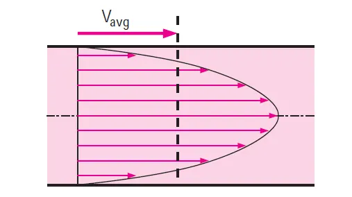
It can be seen that the velocity profile across the pipe is parabolic.
As stated in the above paragraph, as we move from the surface of the wall to the centre of the pipe velocity increase, i.e if we consider a fluid layer velcoity of that particular layer will either relativley more than the layer above it and also relativley less than the layer below it. i.e, there is a relative velocity difference between the layers. So in this case the layer with lower velocity drags the layer with higher velocity in a direction opposite to the direction of flow and hence tries to slow down the layer with higher velocity, this results in developing a shear stress between the layers.
Since the layer which is in contact with the wall has zero velocity (No slip condition), shear stress at that particular layer will be highest. As we move to the centre of the pipe the shear stress decreases. It will be lowest at the centre of pipe where the velocity is free stream velocity.
A hypothetical boundary is considered from the entry of fluid into the pipe, it has a thickness which keeps on increasing from the entry to where the velocity reaches 99% of free stream velocity, this hypothetical layer is called as boundary layer. It can be illustrated as follow,
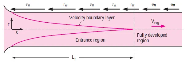
As illsutrated above the velocity profile across the pipe is parabolic, but this paraboic profile is that of a fully developed flow, meaning when fluid starts flowing through the pipe the velocity profile wont to completley parabolic, after a particular distance along the flow direction we can say that the flow is completley developed so this distance strating from the entry of the pipe to a point where the flow is completley developed is a called as Hydrodynamic entry length. From the entry until this distance the velocity profile is not completley parabolic, or in other words the profile is developing. It can be illustrated as follow,
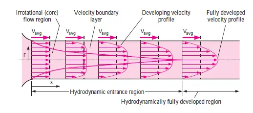
Hydrodynamic entry length's are calculated using a formula, the formula to be used to calculate hydrodynamic entry length varies for a laminar flow as well as for turbulent flow.
For laminar flow, Hydrodynamic entry length, `L_(h) = 0.05*Re*D`
where, `L_(h)` - is hydrodynamic entry length (m)
Re - is Reynolds number
D - is Characteristic length (m), (For internal flow through a pipe characteristic length is nothing but diameter of the pipe)
For turbulent flow, Hydrodynamic entry length, `L_(h) = 1.359*D*(Re)^(1/4)`
where, `L_(h)` - is hydrodynamic entry length (m)
Re - is Reynolds number
D - is Characteristic length (m), (For internal flow through a pipe characteristic length is nothing but diameter of the pipe)
* Also for a viscous flow the shear stress is related to the velocity gradient as, `tau = mu * (delu)/(dely)`
which is also known as newton's law of viscocity
It is essential to understand the above stated flow physics before we dive into setting up the simulations.
# Simulations:
# Setting up the simulation:
Simulation is done using Openfoam. Since it is flow through a cylindrical pipe rather than considering a complete pipe, a small sector with an angle of sweep less than 5 degree is considered and this particular sector is meshed and boundary conditions are applied and then icoFoam solver is used to run the simulation.
# Creating the geometry:
*In openFoam creating a geometry means editing the blockMeshDict file to create the required geometry. This blockMeshDict file is created in matlab using file parsing.
Flow of water at 25 °C entering the a pipe of diameter 0.025 m at a velocity of 0.05 m/s is considered for the simulation. Since we have flow condition, very next thing would be to calculate the Reynolds number and determine wether the flow is lamninar or turbulent,
`Re = (U*D)/nu`
Where , Re - Reynolds number
U - Inlet velocity (m/s)
D - characteristic length (m)
`nu` - Kinematic viscosity of water at 25 °C (m^2/s)
at 25 °C kinematic visosity of water, `nu = 0.893*10^-6 (m^2)/s`
Therefore, Re = (0.05*0.025)/0.893*10^-6 = 1399.77 `approx`1400.
For internal flow Re number more than 2300 is considered as turbulent flow. In our calculations we have Re < 2300 and hence the flow is laminar.
We have for laminar flow, Hydrodynamic entry length, `L_(h) = 0.05*Re*D`
Therefore, `L_(h) = 0.05*1400*0.025 = 1.75`
i.e, from the inlet till a length of 1.75 meters the flow is not completley developed, so a 0.75 m extra length is provided so that it is possible to plot velocity profile of completley developed flow. Therefore the total length of pipe is taken as 1.75 + 0.75 = 2.5 m
* Sector which is to be created using blockMeshDict file, has a sweep angle less than 5° since the angle is small the the arc can be approximated to a straight line, it can be illustrated as follow,
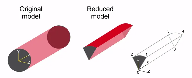
so the co-ordinates for the vertices of the vector is calculated using the trignometric functinons, `y = d/2 * cos(theta/2)` and `z = d/2 * sin(theta/2)`it can be illustrated in a simple way as follow,
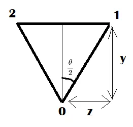
In this simulation angle of 2° is taken accordingly the blockMeshDict file is created by file parsing in matlab.
Boundaries incuded are - inlet, outlet both which are of type patch
- Front and back which are of type wedge
- No slip wall which is of type wall
- axis which is of type empty
Codes for the same is as shown below,
clear all
close all
clc

% Creating blockMeshDict file for wedge creation;

% Defining the Diameter of pipe in meters;
D = 0.025;

% U = 0.05 m/s , nu = 0.893e-06, D = 0.025 m
% R = 0.05*0.025/0.893*e-06
% Defining the reynolds number considering a laminar flow
R = 1400;

% Defining the length of the pipe;
% L = L_h + tol, Length is hrydrodynamic entry length plus a tolerance;
% L_h = 0.05*R*D;

L = (0.05*R*D)+0.75;

% Defining the wedge angle(Degree);
theta = 2;

% Defining the co-ordiantes for wedge creation;
z = (D/2)*sind(theta/2);
y = (D/2)*cosd(theta/2);

% Defining grading factor along x,y and z direction;
g_x = 1;
g_y = 0.1;
g_z = 1;


% File parsing for BlockMeshDict file;

f1 = fopen('output.txt','w');

% Header creation;
fprintf(f1,'%s','/*--------------------------------*- C++ -*----------------------------------*\');
fprintf(f1,'\n');
fprintf(f1,'%s','  =========                 |');
fprintf(f1,'\n');
fprintf(f1,'%s','  \\      /  F ield         | OpenFOAM: The Open Source CFD Toolbox');
fprintf(f1,'\n');
fprintf(f1,'%s','   \\    /   O peration     | Website:  https://openfoam.org');
fprintf(f1,'\n');
fprintf(f1,'%s','    \\  /    A nd           | Version:  6');
fprintf(f1,'\n');
fprintf(f1,'%s','     \\/     M anipulation  |');
fprintf(f1,'\n');
fprintf(f1,'%s','\*---------------------------------------------------------------------------*/');
fprintf(f1,'\n');
fprintf(f1,'%s','FoamFile');
fprintf(f1,'\n');
fprintf(f1,'%s','{');
fprintf(f1,'\n');
fprintf(f1,'%s','    version     2.0;');
fprintf(f1,'\n');
fprintf(f1,'%s','    format      ascii;');
fprintf(f1,'\n');
fprintf(f1,'%s','    class       dictionary;');
fprintf(f1,'\n');
fprintf(f1,'%s','    object      blockMeshDict;');
fprintf(f1,'\n');
fprintf(f1,'%s','}');
fprintf(f1,'\n');
fprintf(f1,'%s','// * * * * * * * * * * * * * * * * * * * * * * * * * * * * * * * * * * * * * //');
fprintf(f1,'\n');
fprintf(f1,'\n');
fprintf(f1,'%s','convertToMeters 1;');
fprintf(f1,'\n');
fprintf(f1,'\n');

% vertice creation;
fprintf(f1,'%s','vertices');
fprintf(f1,'\n');
fprintf(f1,'(\n');
fprintf(f1,'    (%d %d %d)\n',0,0,0);
fprintf(f1,'    (%d %d %d)\n',0,y,z);
fprintf(f1,'    (%d %d %d)\n',0,y,-z);
fprintf(f1,'    (%d %d %d)\n',L,0,0);
fprintf(f1,'    (%d %d %d)\n',L,y,z);
fprintf(f1,'    (%d %d %d)\n',L,y,-z);
fprintf(f1,');\n\n');

% Block creation;
fprintf(f1,'blocks\n');
fprintf(f1,'(\n');
fprintf(f1,'    hex (0 3 5 2 0 3 4 1) (400 60 1) simpleGrading (%d %d %d)\n',g_x,g_y,g_z);
fprintf(f1,');\n\n');

% Edge creation;
fprintf(f1,'edges\n');
fprintf(f1,'(\n');
fprintf(f1,'    arc 1 2 (0 %d 0)\n',D/2);
fprintf(f1,'    arc 4 5 (%d %d 0)\n',L,D/2);
fprintf(f1,');\n\n');

% Boundary creation;
fprintf(f1,'boundary\n');
fprintf(f1,'(\n');

%inlet face;
fprintf(f1,'    inletwall\n');
fprintf(f1,'    {\n');
fprintf(f1,'        type patch;\n');
fprintf(f1,'        faces\n');
fprintf(f1,'        (\n');
fprintf(f1,'            (2 0 0 1)\n');
fprintf(f1,'        );\n');
fprintf(f1,'    }\n');

%Outlet face;
fprintf(f1,'    outletwall\n');
fprintf(f1,'    {\n');
fprintf(f1,'        type patch;\n');
fprintf(f1,'        faces\n');
fprintf(f1,'        (\n');
fprintf(f1,'            (4 3 3 5)\n');
fprintf(f1,'        );\n');
fprintf(f1,'    }\n');

%Top face;
fprintf(f1,'    Noslipwall\n');
fprintf(f1,'    {\n');
fprintf(f1,'        type wall;\n');
fprintf(f1,'        faces\n');
fprintf(f1,'        (\n');
fprintf(f1,'            (5 2 1 4)\n');
fprintf(f1,'        );\n');
fprintf(f1,'    }\n');

%wedge front;
fprintf(f1,'    front\n');
fprintf(f1,'    {\n');
fprintf(f1,'        type wedge;\n');
fprintf(f1,'        faces\n');
fprintf(f1,'        (\n');
fprintf(f1,'            (1 0 3 4)\n');
fprintf(f1,'        );\n');
fprintf(f1,'    }\n');

%wedge Back;
fprintf(f1,'    Back\n');
fprintf(f1,'    {\n');
fprintf(f1,'        type wedge;\n');
fprintf(f1,'        faces\n');
fprintf(f1,'        (\n');
fprintf(f1,'            (2 5 3 0)\n');
fprintf(f1,'        );\n');
fprintf(f1,'    }\n');

%wedge axis;
fprintf(f1,'    axis\n');
fprintf(f1,'    {\n');
fprintf(f1,'        type empty;\n');
fprintf(f1,'        faces\n');
fprintf(f1,'        (\n');
fprintf(f1,'            (0 3 3 0)\n');
fprintf(f1,'        );\n');
fprintf(f1,'    }\n');
fprintf(f1,');\n\n');


%Patchpairs;
fprintf(f1,'mergePatchPairs\n');
fprintf(f1,'(\n');
fprintf(f1,');\n\n')

fprintf(f1,'// ************************************************************************* //');

fclose(f1);
When above matlab codes are run we get a text file 'output.txt' as output, which is nothing but the blockMeshDict file, this file is copied inside the system directory of icoFoam case setup.
BlockMeshDict file generated from the above code is as shown below:
/*--------------------------------*- C++ -*----------------------------------*\
  =========                 |
  \\      /  F ield         | OpenFOAM: The Open Source CFD Toolbox
   \\    /   O peration     | Website:  https://openfoam.org
    \\  /    A nd           | Version:  6
     \\/     M anipulation  |
\*---------------------------------------------------------------------------*/
FoamFile
{
    version     2.0;
    format      ascii;
    class       dictionary;
    object      blockMeshDict;
}
// * * * * * * * * * * * * * * * * * * * * * * * * * * * * * * * * * * * * * //

convertToMeters 1;

vertices
(
    (0 0 0)
    (0 1.249810e-02 2.181551e-04)
    (0 1.249810e-02 -2.181551e-04)
    (2.500000e+00 0 0)
    (2.500000e+00 1.249810e-02 2.181551e-04)
    (2.500000e+00 1.249810e-02 -2.181551e-04)
);

blocks
(
    hex (0 3 5 2 0 3 4 1) (400 60 1) simpleGrading (1 1.000000e-01 1)
);

edges
(
    arc 1 2 (0 1.250000e-02 0)
    arc 4 5 (2.500000e+00 1.250000e-02 0)
);

boundary
(
    inletwall
    {
        type patch;
        faces
        (
            (2 0 0 1)
        );
    }
    outletwall
    {
        type patch;
        faces
        (
            (4 3 3 5)
        );
    }
    Noslipwall
    {
        type wall;
        faces
        (
            (5 2 1 4)
        );
    }
    front
    {
        type wedge;
        faces
        (
            (1 0 3 4)
        );
    }
    Back
    {
        type wedge;
        faces
        (
            (2 5 3 0)
        );
    }
    axis
    {
        type empty;
        faces
        (
            (0 3 3 0)
        );
    }
);

mergePatchPairs
(
);

// ************************************************************************* //
All the above boundary conditions are included in the velocity (U) and pressure (p) files which are present in the 0 directory of the case setup, both the files are included below:
Pressure file:
/*--------------------------------*- C++ -*----------------------------------*\
  =========                 |
  \\      /  F ield         | OpenFOAM: The Open Source CFD Toolbox
   \\    /   O peration     | Website:  https://openfoam.org
    \\  /    A nd           | Version:  6
     \\/     M anipulation  |
\*---------------------------------------------------------------------------*/
FoamFile
{
    version     2.0;
    format      ascii;
    class       volScalarField;
    object      p;
}
// * * * * * * * * * * * * * * * * * * * * * * * * * * * * * * * * * * * * * //

dimensions      [0 2 -2 0 0 0 0];

internalField   uniform 0;

boundaryField
{
    inletwall
    {
        type            zeroGradient;
    }

    outletwall
    {
        type            fixedValue;
        value           uniform 1;
    }

    Noslipwall
    {
        type            zeroGradient;
    }

    front
    {
        type            wedge;
    }

    Back
    {
        type            wedge;
    }

    axis
    {
        type            empty;
    }
}

// ************************************************************************* //
Velocity file:
/*--------------------------------*- C++ -*----------------------------------*\
  =========                 |
  \\      /  F ield         | OpenFOAM: The Open Source CFD Toolbox
   \\    /   O peration     | Website:  https://openfoam.org
    \\  /    A nd           | Version:  6
     \\/     M anipulation  |
\*---------------------------------------------------------------------------*/
FoamFile
{
    version     2.0;
    format      ascii;
    class       volVectorField;
    object      U;
}
// * * * * * * * * * * * * * * * * * * * * * * * * * * * * * * * * * * * * * //

dimensions      [0 1 -1 0 0 0 0];

internalField   uniform (0 0 0);

boundaryField
{
    inletwall
    {
        type            fixedValue;
        value           uniform (0.05 0 0);
    }

    outletwall
    {
        type            zeroGradient;
    }

    Noslipwall
    {
        type            fixedValue;
        value           uniform (0 0 0);
    }

    front
    {
        type            wedge;
    }

    Back
    {
        type            wedge;
    }

    axis
    {
        type            empty;
    }
}

// ************************************************************************* //
Since inlet velocity of water is 0.05 m/s, same is provided in the U file as shown above.
* Total time until which the simulations to be run is calculated,
we have , `V = l/t`
`v = 0.05 m/s`
`l = 2.5 m`
Therefore, t = 2.5/0.05 = 50 sec, which implies at a velocity of 0.05 m/s fluid takes 50 sec to complete one pass.
So total time of 50 sec is provided in the controlDict file, time step is determined using trial and error method. In this case time step delta t = 0.007 sec is used under which the courant number is well under the max value of C = 1. Below is the controlDict file:
/*--------------------------------*- C++ -*----------------------------------*\
  =========                 |
  \\      /  F ield         | OpenFOAM: The Open Source CFD Toolbox
   \\    /   O peration     | Website:  https://openfoam.org
    \\  /    A nd           | Version:  6
     \\/     M anipulation  |
\*---------------------------------------------------------------------------*/
FoamFile
{
    version     2.0;
    format      ascii;
    class       dictionary;
    location    "system";
    object      controlDict;
}
// * * * * * * * * * * * * * * * * * * * * * * * * * * * * * * * * * * * * * //

application     icoFoam;

startFrom       startTime;

startTime       0;

stopAt          endTime;

endTime         50;

deltaT          0.007;

writeControl    timeStep;

writeInterval   20;

purgeWrite      0;

writeFormat     ascii;

writePrecision  6;

writeCompression off;

timeFormat      general;

timePrecision   6;

runTimeModifiable true;


// ************************************************************************* //
* TransportProperties is a file in the constant directory of the case setup where the value of kinematic viscosity of fluid is provided, as mentioned above in this case since the fluid is water flowing throuh pipe at 25 °C the kinematic viscosity, `nu = 0.893*10^-6 m^2/s` is provided. Below is a grab of the same
/*--------------------------------*- C++ -*----------------------------------*\
  =========                 |
  \\      /  F ield         | OpenFOAM: The Open Source CFD Toolbox
   \\    /   O peration     | Website:  https://openfoam.org
    \\  /    A nd           | Version:  6
     \\/     M anipulation  |
\*---------------------------------------------------------------------------*/
FoamFile
{
    version     2.0;
    format      ascii;
    class       dictionary;
    location    "constant";
    object      transportProperties;
}
// * * * * * * * * * * * * * * * * * * * * * * * * * * * * * * * * * * * * * //

nu              [0 2 -1 0 0 0 0] 0.893e-6;


// ************************************************************************* //
*other than the above mentioned files there are OpenFoam files such as fvsolution and fvschemes which is required to run the simulation but no changes are done on these fies and they are used as such it is there in the case setup.
* Once all the above files are set, blockMesh is typed in the command window to generate the mesh. The mesh so generated can be viewed in the postprocessing tool ParaView. After that checkMesh command can be used to check wether the mesh is ok. Once both of the above commands runs without any error we can run the simulation by typing icoFoam in the command window. After successfully running the simulation the result obtained is viewed and postprocessed in paraView.
* Since we are simulating for a small sector, it is not possible to obtain the complete velocity profile. so the sector is mirrored using reflect option present in paraView. When did we get our sector under consideration mirrored along the axis hence complete velocity profile can be obtained.
# Velcoity contour plot:
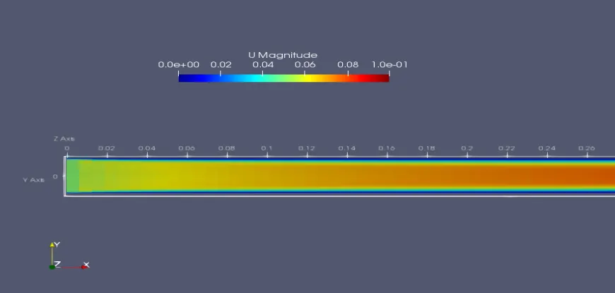
Below is the velocity contour plot that is obtained along the length of the pipe,
*Inlet:
* Outlet
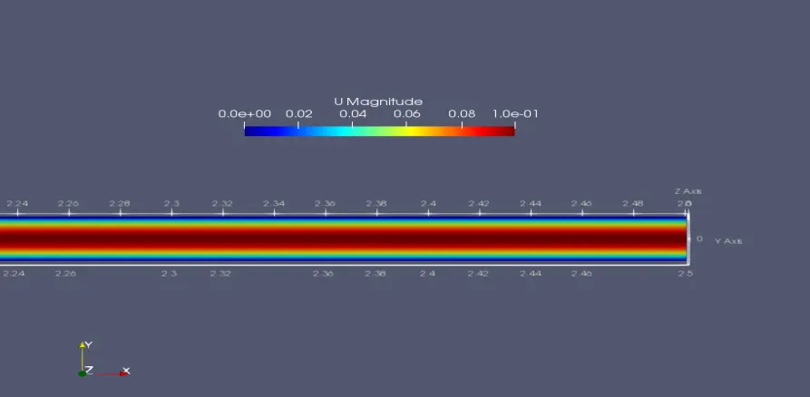
* so it can be observed that we started with inlet velocity of 0.05 m/s and we got final velocity 0.1 m/s. Also near the walls the velocity is zero and it is increasing to the centre of the pipe. which seems to be pretty much as per the flow physics.
* To further validate the result we can take the velocity profile along the radial direction of the pipe.
# Velcoity profiles along radial directions:
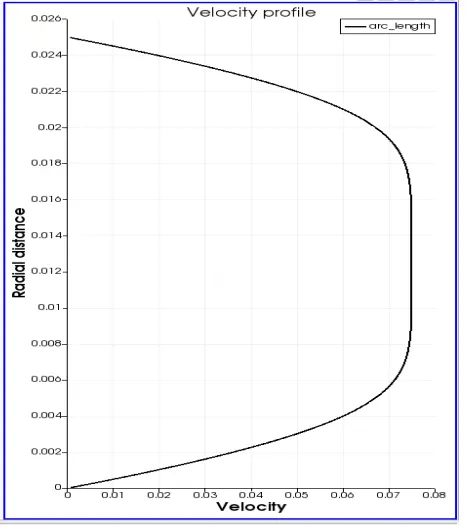
* Since from the above calculations we have obtained hydrodynamic entry length, `L_(h) = 1.75 m` so if we take plot of velocity profiles till this point it should be a developing parabola rather than a complete parabola.
For this we can use plotover line tool of the paraView, which provides us with a line probe. This line probe is placed at different points along the length of the pipe and hence the velocity profile is plotted.
So in here we will start with a distance of 0.25 m from the entry, having a increment of 0.5 m till a point 2.25 m away from the entry.
* At a distance of 0.25 m from the inlet:
* At a distance of 0.75 m from the inlet:
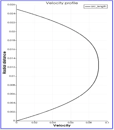
* At a distance of 1.25 m from the inlet:
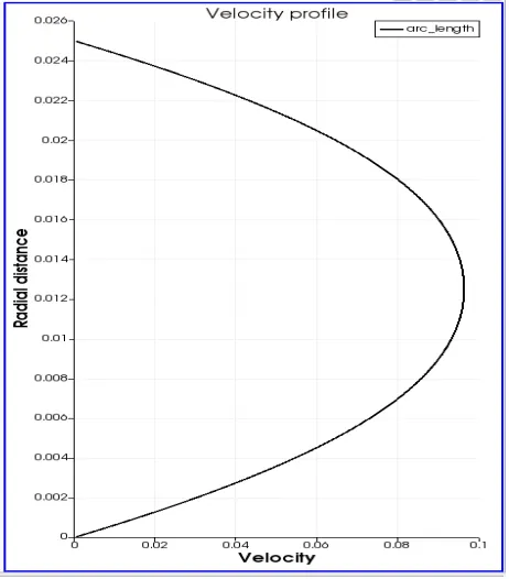
* At a distance of 1.75 m from the inlet:
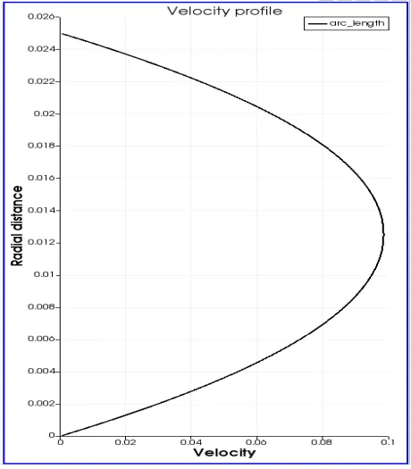
* At a distance of 2.25 m from the inlet:
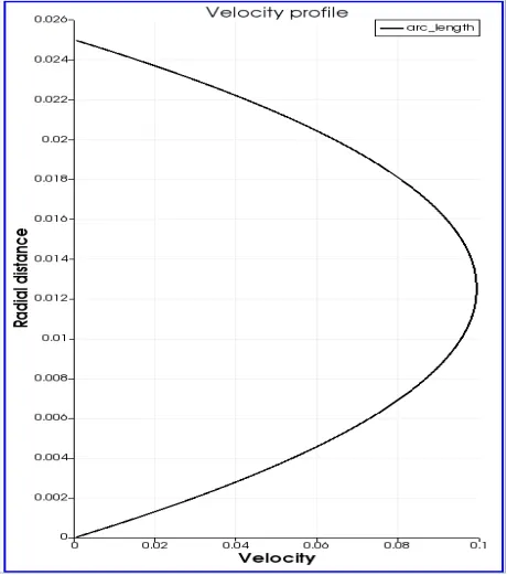
* It is evident from the above velocity profiles that till the hydrodynamic length of 1.75 m is reached the parabola was not complete or in other words the flow was not fully developed, after this at a point 2.25 m from the inlet where the flow is completley develloped it can be observed that the parabola is complete or in other words the flow is fully developed. Hence we can conclude that we have validated our results and it matches with the flow physics.
velocity profile being validated, now we can plot the shear stress.
# Plot of shear stress:
Plotting shear stress is not straight forward as plotting the velocity profile. Because in paraView tau is not calcuated directly, so it becomes relevant that we firts calculate tau and then use plot overline command to plot the shear stress.
We have newton's law for viscous flow, `tau = mu * (delu)/(dely)` this can be used to calculate the shear stress. Steps of calculation are listed below.
1. We need to calculate magnitude of vector U, this can be achieved using the mag option present in the calculator. If we provide mag(U) in the calculator we will get the magnitude of velocity.
2. Once magnitude of velocity is computed next step is to calculate its gradient, this can be achieved by inserting gradient of unstructured data set, this is a computational option present in the paraview. once this option is inserted from filters we can provide the calculated velocity gradient as input and hence the gradient of velocity can be calculated.
3. Once the gradient is calculated, dynamic viscosity of water at 25 °C is multiplied, `mu = 0.000890 (kg)/(m*s)`hence tau is calculated.
Using plotover line the line probe can be placed anywhere along the radial direction and shear plot can be obtained,
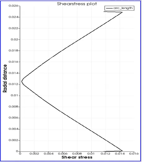
* It can observed in the plot, that shear stress experienced by layers adjacent to the wall is more.
* As we move along the radial direction the shear stress keeps decreasing and at the centre where the velocity is free stream velocity shear stress is almost zero.