Ahmed Body Challenge
# Aim of the project is to simulate a turbulent flow past a Ahmed body and hence calculate coefficient of drag and coefficient of lift. Also to understand flow separation and understand how wake forms and how it affects the flow. also to perform grid independency test.
# Introduction:
Ahmed body is a geometry which represents a generic car body. We can consider it as a blunt body which has a rough geometry resemblance that of a car, it was first developed and experimented by s.r Ahmed and hence it is named as ahmed body. Significance of an ahmed body is that, suppose we have developed a CFD code, which we need to run simulations around a new model car which is to be developed, so in that case we can use ahmed body to check whether the codes that were developed is good. We can use the codes and run simulations around a ahmed body to capture flow parameters in a turbulent flow. If we are able to validate the numerical results then we can use the codes to develop the new model car.
Below is a typical illustration of a ahmed body:
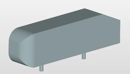
Ahmed body used in this simulation is as shown below,
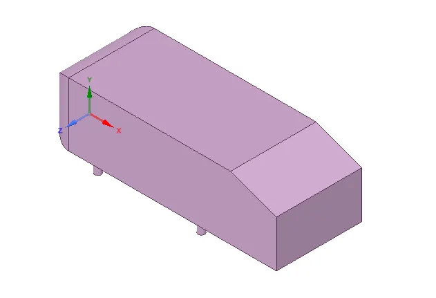
which is of following dimensions, in meters
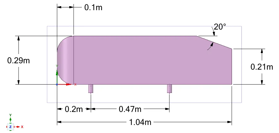
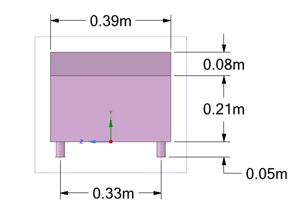
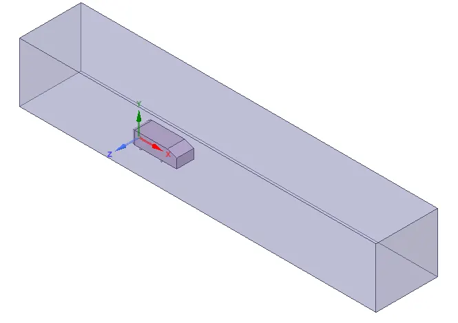
To run external flow simulations on any body wind tunnels are used, same is followed in industries. So in here we provide an enclosure to the ahmed body which acts as a wind tunnel.
A screen shot of the same is shown below:
the dimensions which is followed is as shown below,
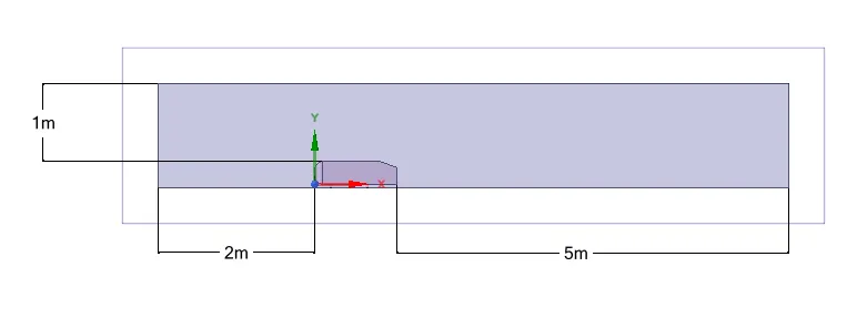
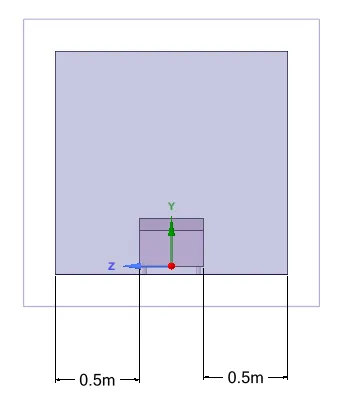
once geometry is prepared to this extent in spaceclaim it is given a base mesh using the meshing interface of ansys and simulations are run for 100 iterations, velocity contour and pressure contour plots are taken in the fluent. Since the base line mesh is very coarse, from the velocity contour we will get a rough picture of wake region formed, so based on this one more enclosure is provided. Similar practice is followed in industries while running external flow simulations.
when inner enclosure is provided, the whole setup looks as follow:
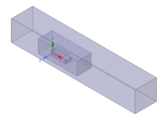
which is of following dimensions:
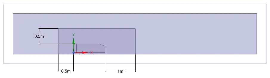
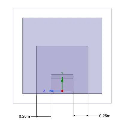
we can mesh the above setup and it can be used for simulations, but meshing the whole setup will increase the number of cells, so as an alternative since the whole setup is completley symmetric the setup is split and share topology option is used so that information between the cells get shared. When splitted the whole setup looks like below.
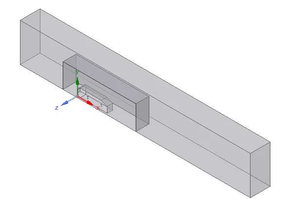
this splitted half is meshed in the meshing interface.
# Meshing:
* First base line mesh is added to the whole geometry, when meshed it looks as follow,
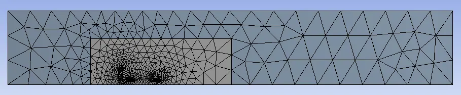
* The outer enclosure is provided with hexahedral meshes. Hexahedral meshes are the ones which are better than tetrahedral meshes, but we cannot use hexahedral meshes as such because it wont fit into complex geometries which involves curves and acute angles. When complex geometries are meshed tetrahedral can be preffered. If we observe the outer enclosure we can see that it is just a simple geometry involving only lines and hence hexahedral meshes can be used.
Hexahedral meshes are added using the method option where multizone option is used to mesh the outer enclosure with hexahedral mesh. Along with adding hexahedral meshes to the enclosure the mesh element size is reduced from 419 mm (above base line mesh) to 100 mm.
* Inner enclosure will have the typical base line tetrahedral meshes, in here the element size of the mesh is reduced using the sizing option and hence a element size of 30 mm is used for the meshes of inner enclosure. When meshed it looks like,

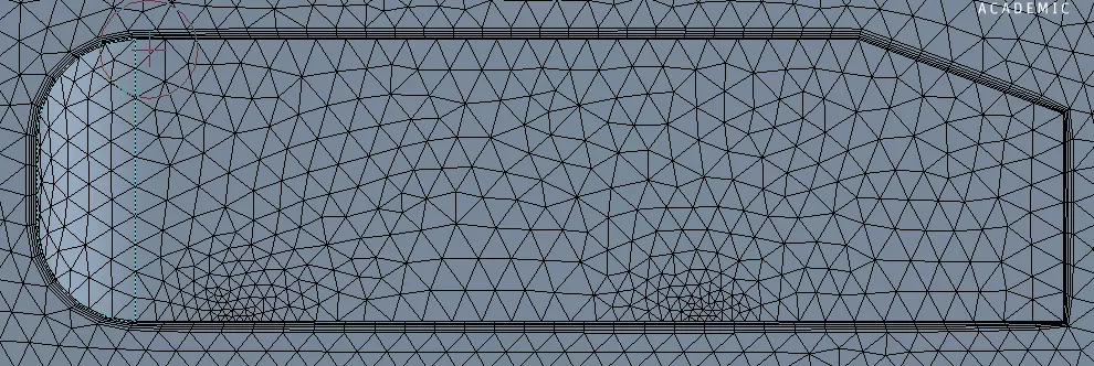
* Since we are interested in capturing wall phenomena, it will be better if we add inflation layers above ahmed body (car_wall). Inflation layers are also called as body fitted mesh, it helps in capturing gradient normal to the wall with minimum number of cells.
* While adding inflation layers one of the important aspect that is being taken care is calculation of first layer thickness. This is achieved using y+.
Before starting with first layer thickness calculation, let us start with reynolds number calculations,
Reynolds number, `Re = (rho*V*L)/mu`
`rho` - Density of fluid (kg/m^3)`
V - Velocity of fluid (m/s).
L - Characteristic length of the body (m).
`mu` - Dynamic viscosity of fluid (kg/m*s)`
In our case we are using air as fluid, with inlet velocity , V = 25 m/s
L = 1.04 m, which is length of ahmed body.
`rho` = 1.225 kg/m^3
`mu` = 1.7894 e -05 kg/m*s
therefore, Re = (1.225*25*1.04)/1.7894 e-05 = 1.77 e 06, since Re is above 2 e 05 we can consider the flow as turbulent.
Now coming to first layer thickness calculation, `y+ = (rho*u_(tau)*y)/mu`
so from the above we can wirte, `y = (mu*(y+))/(rho*u_(tau))`
where, y is the first layer thickness
`u_(tau) = sqrt(tau_(w)/rho`
`tau_(w)` - Wall shear stress (N/m^2)
wall shear stress , `tau_(w) = 1/2*C_(f)*rho*V^2`
where, `C_(f)` - Skin friction
Skin friction, `C_(f) = 0.058*Re^-0.2`
To understand what should be the value of y+ that we need to select so that we can calculate the value of first layer thickness and total thickness correctly, it is essential to understand the below plot,
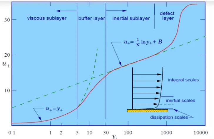
from the above plot the red solid line represnts the variation of u+ w.r.t y+ obtained from DNS, the dotted green line is obtained from respectve formula's as shown in the plot,
it can be observed that between 5<y+<30, the result does not match with the DNS results and hence that region should be completley avoided.
In this simulation, y+ = 325 is taken and first layer thickness is calculated, using the formual
`y = (mu*(y+))/(rho*u_(tau))``
so first we need to calculate the wall shear stress, `tau_(w) = 1/2*C_(f)*rho*V^2`
`C_(f) = 0.058*Re^-0.2`
we have, Re = 1.77 e 06.
therefore, `C_(f)` = 0.058*(1.77 e 06)^-0.2
= 3.242 e -03
now we can calculate `tau_(w) = 1/2*C_(f)*rho*V^2`
`tau_(w)` = 1/2*3.242 e -03*1.225*(25)^2
= 1.241 N/m^2
we have, `u_(tau) = sqrt(tau_(w)/rho`
`u_(tau) = sqrt(1.241/1.225)` = 1.006`
so first layer thickness , y = (1.7894 e-05*325) / (1.225*1.009) = 4.7 mm
Total of 5 inflation layers are used with a growth rate of 1.2, hence total thickness = 4.7*(1.2)^5 = 11.69 mm
So the above value of total thickness is entered in the inflation options and hence we get inflation layers as shown below,
# Simulations:
Ahmed body which is meshed as shown above is used for the simulation. Steady state simulation is used , since the flow is turbulent K-ε turbulent model is used.
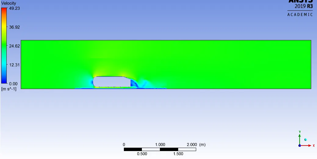
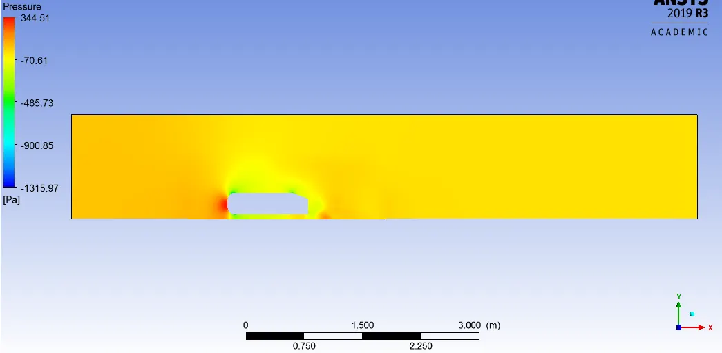
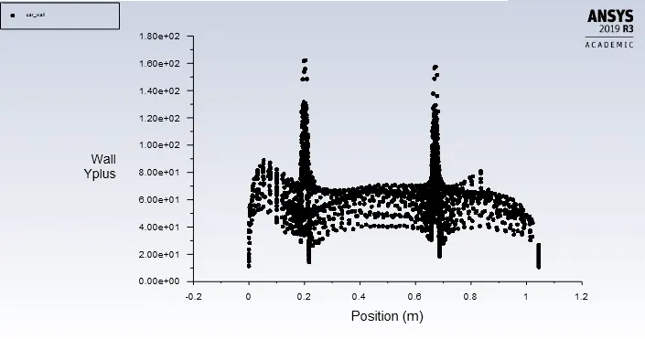
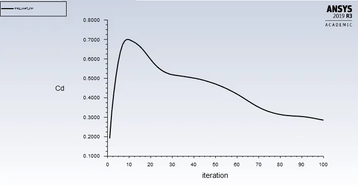
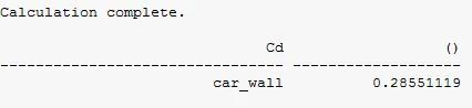
Simulations are run for 100 iterations, coefficient of drag is calculated. Below are the plots obtained from the simulations.
* Velocity contour:
* Pressure contour:
* Y+plot:
* Plot of drag coefficient:
drag coefficient value obtained after simulation is as follow,
* Explaination:
* From the velocity contour we can clearly observe the wake region. To understand how wake region is formed it is essential to understand what is flow separation and on what condition flow separation takes place.
* A flow from high pressure to low pressure (dp/dx < 0) region is always considered as favourable flow, in this case the fluid which is flowing will be decelarated by the skin friction or wall shear stress but the pressure gradient accelarates the flow.
* A flow where there is no pressure gradient (dp/dx = 0) there will be only decelaration because of skin friction.
* Thrid case is where the fluid flows from a low pressure region to high pressure region i.e, dp/dx > 0. This is also known as adverse pressure gradient, when fluid flows under such condition both the pressure gradient as well as skin friction tries to decelarate the flow.
* Flow separation is said to happen when the fluid flow near the wall comes to rest. These are those layers of fluid which are not on the wall but near to the wall, on the wall the layers are at rest which is called as no-slip condition.
* So if there is a flow separation then it's because the layers near the wall have come to rest.
* This can be explained by considering the velocity along y direction, velocity of the fluid at a distance dy from the wall can be given using the taylor series expansion
`u_(y+dy) = u_(y=0)+((delu)/(dely))_(y=0)*deltay`
as we know when flow separation takes place the layer near the wall comes to rest, i.e, `u_(y+dy) = 0`
because of no-slip condition the layer on the wall will be at rest, i.e, `u_((y=0)) = 0`
so we get `((delu)/(dely)) = 0`, and hence this is the condition for flow separatio`
Under such condition where `((delu)/(dely)) = 0` the layers near the wall resist's to flow in the direction of wall and hence flows in the opposite direction. where there is backward flow that region of flow is called wake.
For a flow from high pressure to low pressure i.e dp/dx < 0 since pressure gradient accelarates the fluid flow there wont be any reverse flow, same holds good for zero pressure gradient flow.
But for adverse pressure gradient flow i.e, dp/dx > 0, the pressure gradient decelarates the fluid flow so chances for flow separation and wake formation is more.
This can be further explained using the x-momentum equation for boundary layer flow, which is given as follow
`u*(delu)/(delx)+v*(delu)/(dely) = -(1/rho)*(dp)/(dx)+(mu/rho)*(del^2u)/(dely^2)`
if we apply this equation at wall i.e, y = 0, we have at y = 0, u = 0 and v = 0. if we consider a pressure gradient across the flow then above equation can be written as
`(1/mu)*(dp)/(dx) =(del^2u)/(dely^2)`
a) dp/dx < 0, favourable flow condition we will have `(del^2u)/(dely^2) < 0`
b) dp/dx = 0 , `(del^2u)/(dely^2) = 0`
c) dp/dx > 0, `(del^2u)/(dely^2) >0`
plot of u along y is as shown below for the above conditions,
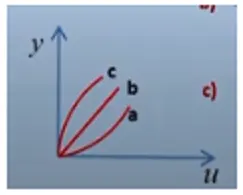
above plots a, b, c can be used to get the profile of velocity at y=0 at different pressure gradients and it is as shown below,

We have condition for flow separation given as `((delu)/(dely)) = 0`, so when velocity gradient becomes zero the wall shear stress becomes zero and hence from this point the flow separartion starts and when adverse pressure gradient is more flow reversal occurs as shown above.
Vector plot showing flow reversal is as shown below,
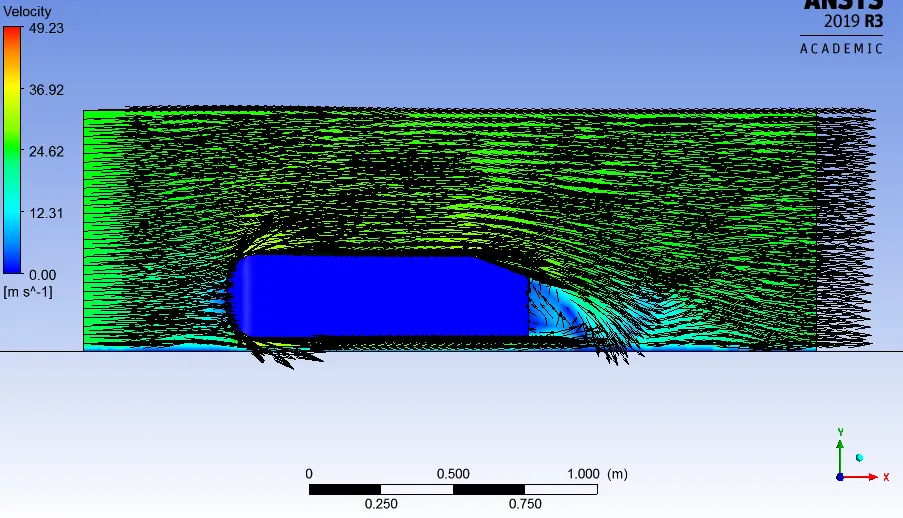
from the above vector plot it can be clearly observed that at wake there is a flow reversal.
* Negative pressure in the wake is because we have set outlet pressure as guage pressure which is zero, since it is a adverse pressure gradient flow, pressure is increasing towards the outlet and hence negative pressure.
# Grid independency test:
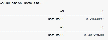
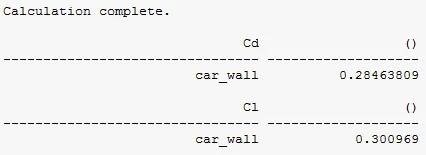
* Grid independency test is performed by changing the value of y+, as y+ is decreased total cell count increases, for each value of y+ simulation is run for 100 iterations and value of coefficient of drag and coefficient of lift at car wall is noted.
1. for y+ = 300, first layer thickness, y = 4.34 mm, total cell count = 328096,
2. for y+ = 250, first layer thickness = 3.61 mm, total cell count = 329120,
3. for y+ = 200, first layer thickness = 2.89 mm, total cell count = 330348,
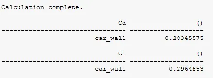
From the above results it is clear that even for different number of cell count the value of drag coefficient as well as lift coefficient remianed almost same, hence the simulation is grid independent.