Challenge on Combustion
AIM
* To perform a combustion simulation on the combustor model and plot the variation of mass fraction of different species in the combustion using line probes.
* To perform combustion simulation by adding water from 5% to 30% in fuel and hence observe the changes in mass fraction of soot and `NO_x` in pollutatnts.
INTRODUCTION
Combustion refers to burning of a substance in the presence of air and hence producing heat and energy. Most commonly seen combustion are combustion of fuels in automobiles. Apart from automobiles there are different applications where fuels are burnt such as in thermal power plants, in ships and aeroplanes to run the propeller and so on. Chemically a combustion is said to be combining of fuel with oxygen and hence producing carbondioxide and water, which can be written stoichometrically as shown below,
`CH_4 + 2*(O_2 + 3.76 N_2) = CO_2 + 2*H_2O + 7.52N_2`
In practical the combustion products are not as simple as `H_2O`and `CO_2` as shown above apart from this there will oxides of nitrogen, oxides of sulphur, soot etc. Apart from water what ever combustion products gets formed are harmfull to the environment as well as to living beings. So it very important that we should stop the formation of these harmfull pollutants or atleast reduce the formation of pollutants to a large extent.
There have been extensive researches done to determine different models to reduce pollutants, one of the research is to inject water along with the fuel into the combustion chamber and hence reduce the formation of soot and `NO_x`. In this simulation this particular approach is used and hence variation in mass fraction of soot and `NO_x` are observed.
In this simulation `CH_4` is the fuel used and combustion simulation is performed inside a modelled cylindrical combustor. In first part of the simulation combustion simulation is performed without adding water with fuel and mass fraction of all the combustion products are noted. In the second part of the simulation water is added along with fuel into the combustion chamber and hence variation in mass fraction of soot and `NO_x`is noted.
SIMULATION
Geometry :
A modelled cylindrical combustor is used to run the simulation, the cylindrical combustor is as shown below,
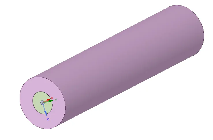
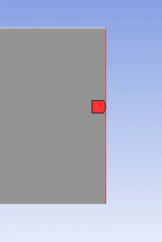
the centre circle represents the fuel inlet and the external circle represents the air intake. Above geometry is splitted along YZ plane and 2D geometry is extracted. The final geometry obtained after splitting is as shown below,
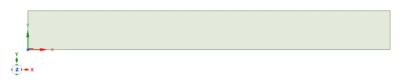
Above geometry is boundary flagged and meshed in the meshing interface of ansys workbench.
Meshing:
Triangular meshes are applied on the geometry using the insert local control. A mesh size of 2 mm is applied along with proximity capture with number of cells along the gap set at 3. Also the boundary's are flagged as,
Fuel_inlet -

Air_inlet -
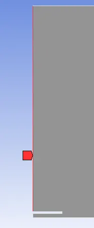
Wall_side -
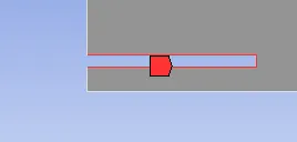
Axis -

Wall -

Outlet -
Meshed surface looks as follow,
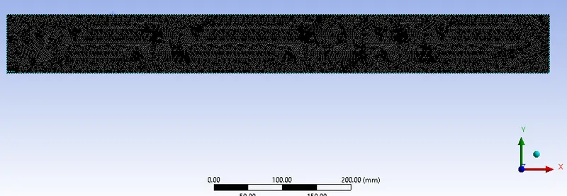
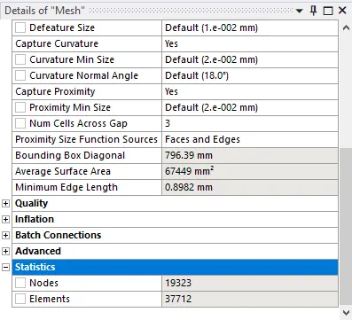
with a total of 37712 cells
Above geometry is imported to fluent and appropriate B.C's are applied and hence combustion is simulated.
Solver setup :
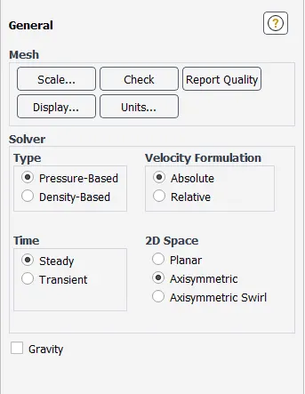
A steady state simulation is performed using a pressure based solver, and a axisymmetric 2D space is set since the geometry is axisymmetric.
* Energy equation is checked so that the heat equation is also solved. Standard K-ε viscous model is used with standard wall function. All other local controls under the viscous model is left as default.
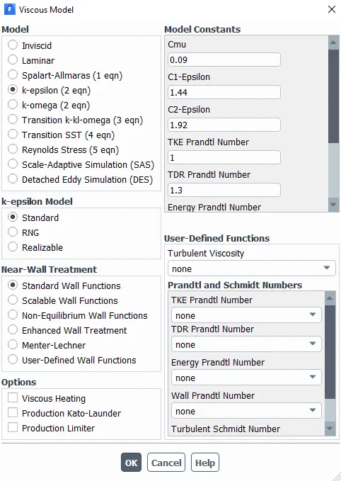
* Using the materials local control methane-air fuel is imported from fluent data base. Main settings required to run the combustion simulation is provided using the species local control.
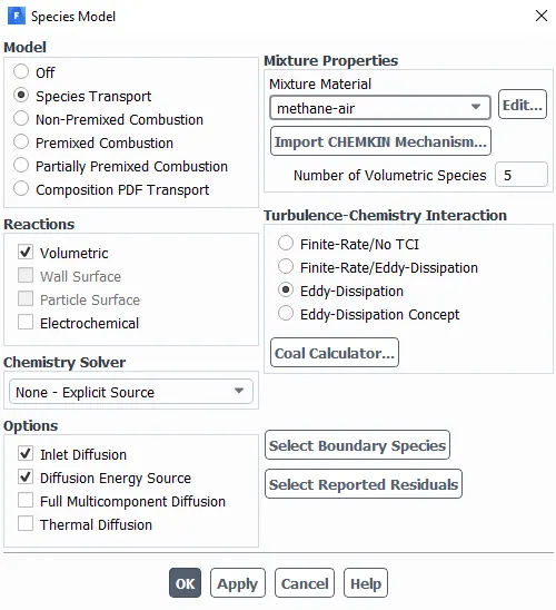
* Model is set to species transport so that species transort equation gets solved. Reaction is set as volumetric, inlet diffusion and diffusion energy source is set as options. Turbulence chemistry interaction is set as Eddy-dissipation. Since methane air is selected as fuel number of volumetric species is auto set to 5.
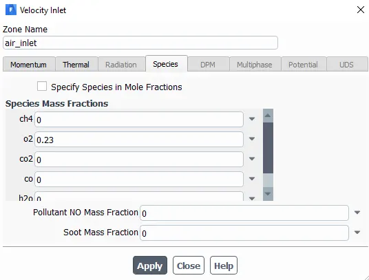
* Under boundary conditions for Air_inlet which is set as velocity inlet, velocity of air is set as 0.5 m/s also the species with which the air is composed of is set as `O_2` with a mass fraction of 0.23.
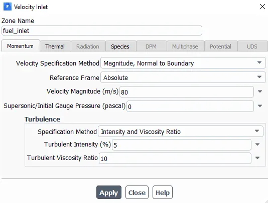
* For Fuel_inlet which is also set as velocity inlet, the inlet fuel velocity is set as 80 m/s. `CH_4` is the species set for the fuel, or in other word we can say fuel consists only `CH_4`with mass fraction set as 1.
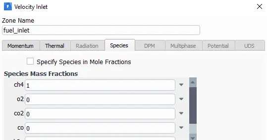
* Outlet boundary type is set as pressure outlet. Boundary's flagged as wall are set as wall type along with no-slip condition. Boundary axis is set as type axis.
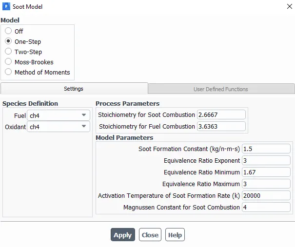
* Also the `NO_x` and soot models needs to be enabled so that these 2 species are considered as the output after combustion.
* `NO_x` and soot can be enabled using the models, for `NO_x` below shown model setup is used.
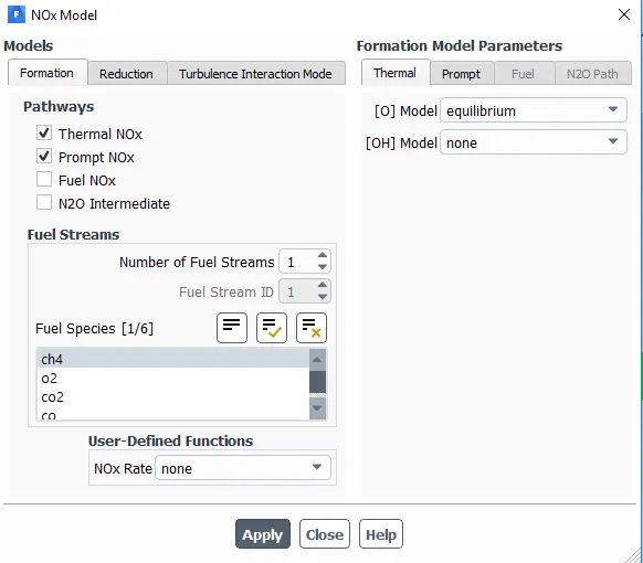
* For soot, one-step model is used
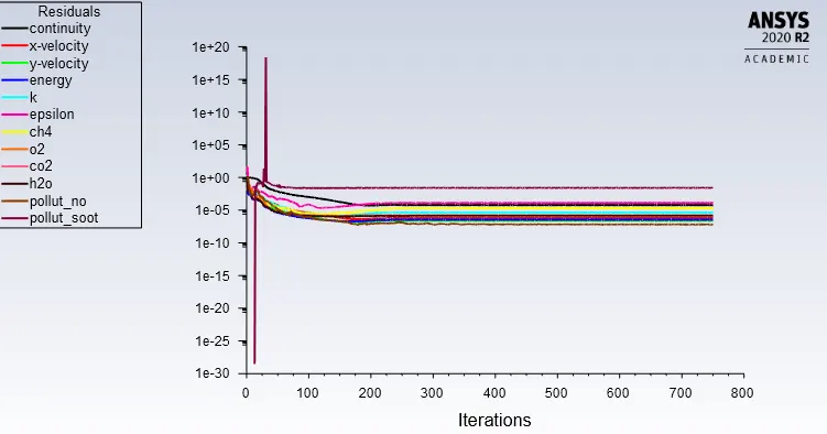
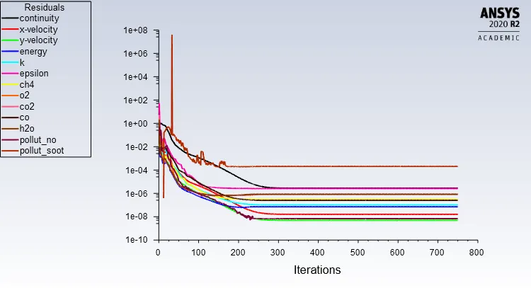
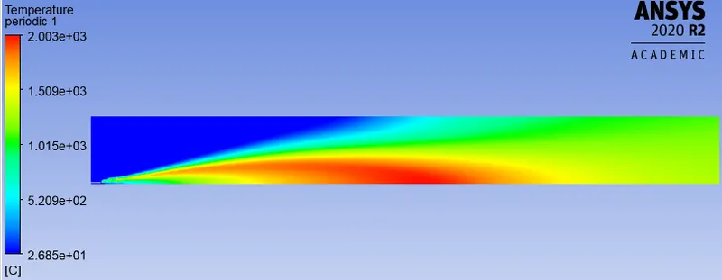
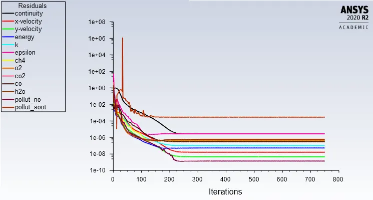
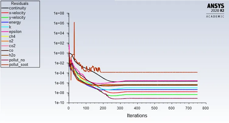
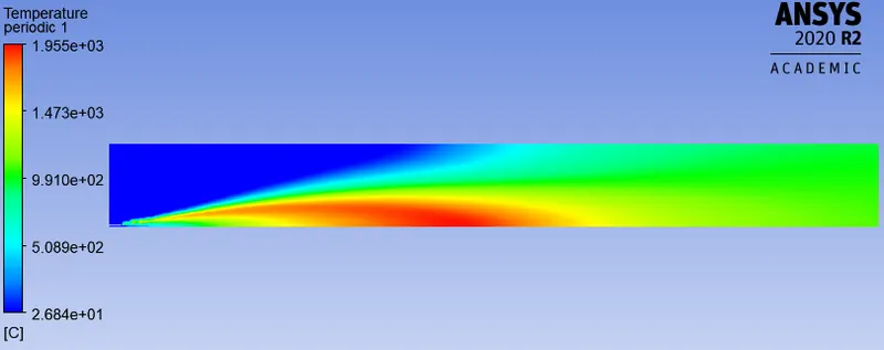
* With above mentioned B.C and settings we can proceed to run the simulation. To get a clear picture of how temperature distribution takes place inside the combustor a temperature contour is added also animation of the same is created. Simulation is run around 750 iterations and the results are noted.
* Residual plot:
* Temperature contour:
* Temperature distribution animation:
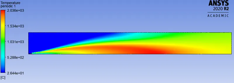
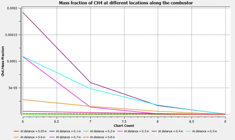
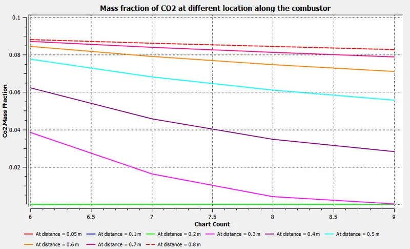
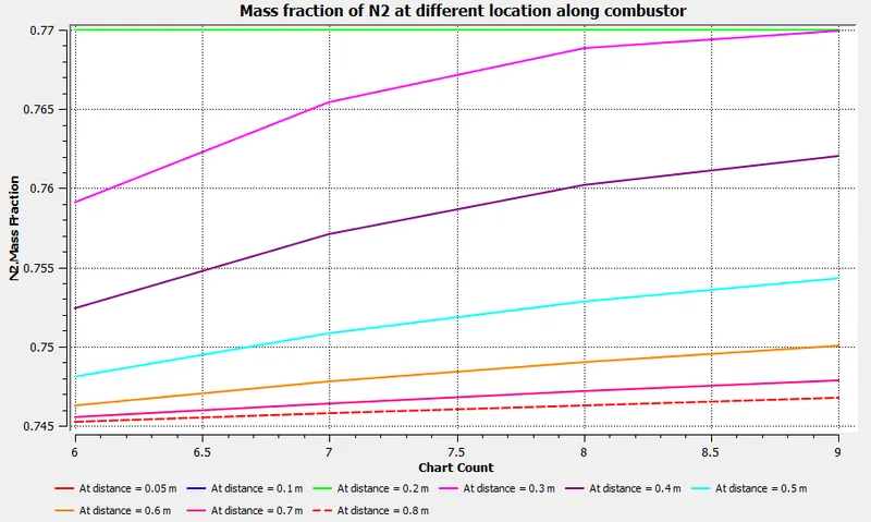
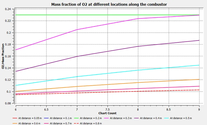
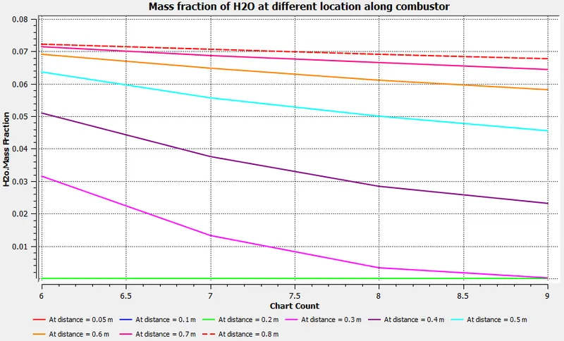
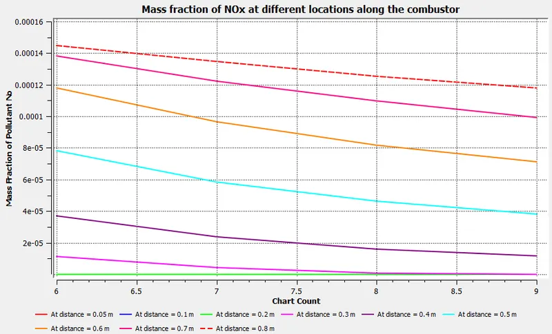
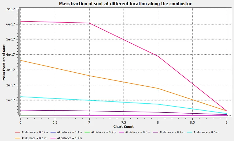
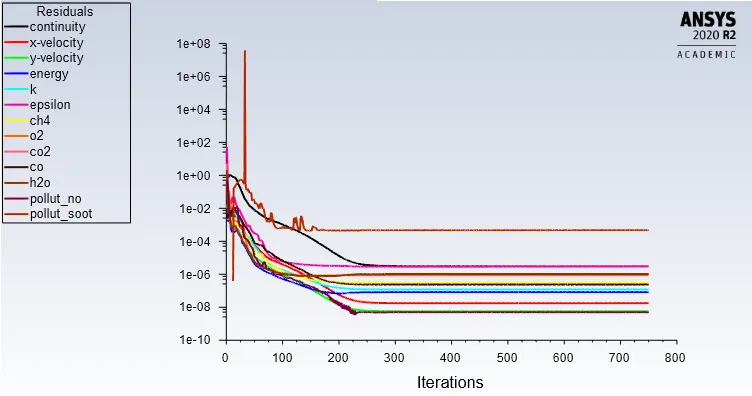
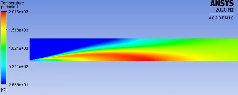
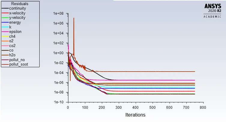
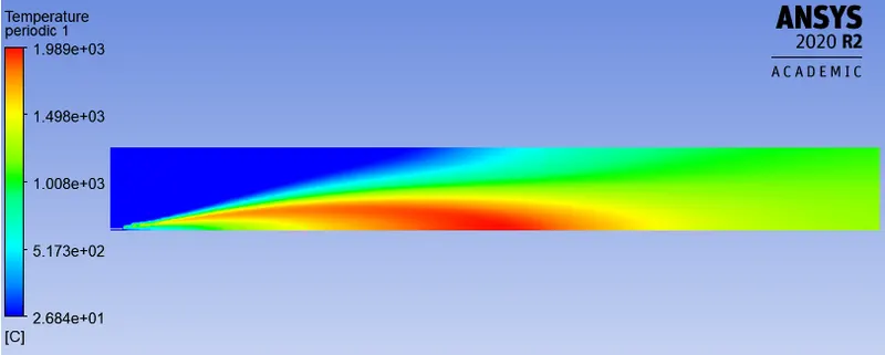
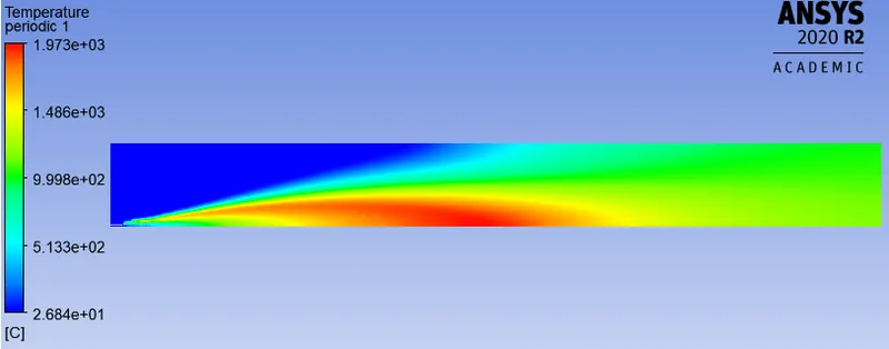
* From the residual plot it is well understood that the solution is converged. Temperature distribution is very much even, max temperature is obtained at the centre of the combustor. At the outlet temperature is moderate. Point of interest for this simulation is to check the variation of mass fraction of different cobustion species such as `CH_4, CO_2, H_2O, N_2, O_2, NO_x, Soot`at different locations along the combustor using a line probe. Line probes are placed at a distance 0.05, 0.1, 0.2, 0.3, 0.4, 0.5, 0.6, 0.7, 0.8 meters along the length of the combustor and mass fraction of each species at above mentioned location are plotted. When all the line probes are placed on the geometry it looks as shown below,

* Mass fraction of `CH_4` :
* Mass fraction of `CO_2`:
* Mass fraction of `N_2`:
* Mass fraction of `O_2`:
* Mass fraction of `H_2O`:
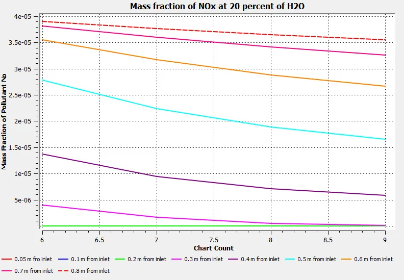
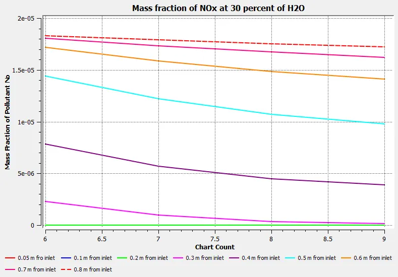
* Mass fraction of `NO_x`:
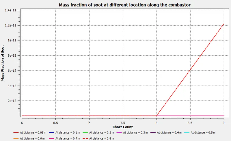
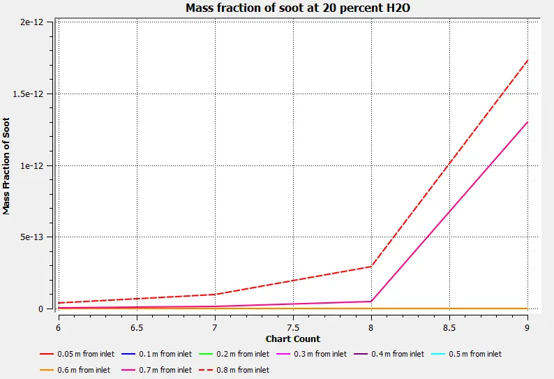
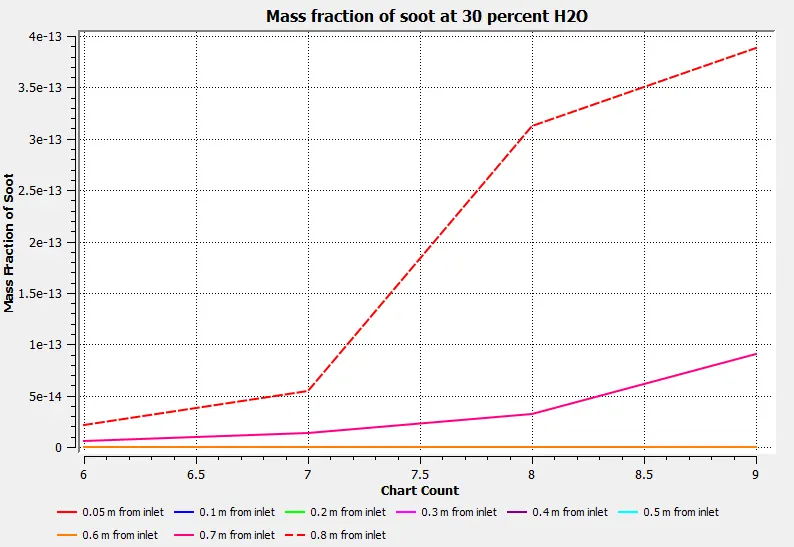
* Mass fraction of soot :
Observation :
* Mass fraction of `CH_4, O_2` are decreasing as we move from inlet side to outlet side at the same time mass fraction of `H_2O, Soot, NO_x, CO_2` are increasing.
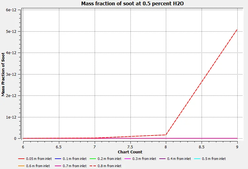
* At outlet increase in mass fraction of soot and `NO_x` is much higher compared to initial stages. Soot formation at outlet is comparativley higher because of which when plot is taken at the outlet, plots concerned at other location gets undermined into a single line.
* Observing the above result which clearly indicates increased formation of soot and `NO_x`at outlet, it becomes relevant that these harmfull pollutants needs to be controlled. Injecting water along with the fuel is approach used to reduce the formation of `No_x` and soot at outlet.
Case 2: Adding water along with fuel to check the formation of soot and `No_x`:
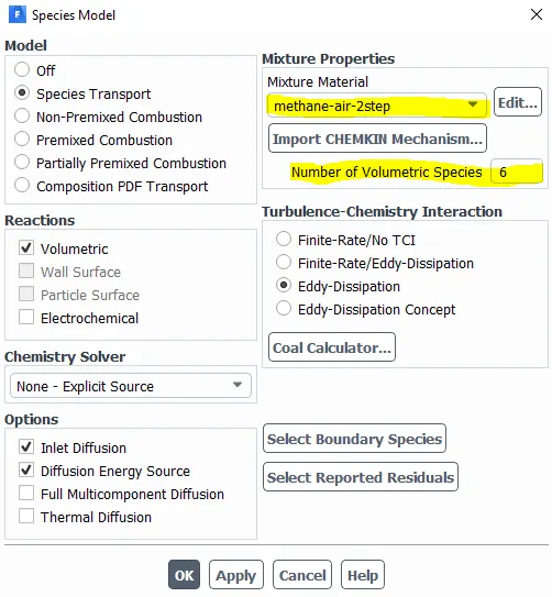
* Same geometry along with the same case setup is used to run the simulation only difference is the fuel material used. In previous case methane-air is the fuel material used whereas in this case methane-air 2 step is used. This material is available in the fluent database and can be copied. In the species local control same material needs to be selected, when this material is set the number of volumetric species gets auto set to 6. A snip of the same is provided below,
* Using methane-air 2 step as the fuel material provides us with an advantage of using water along with fuel. This can be set using the Fuel_inlet boundary,
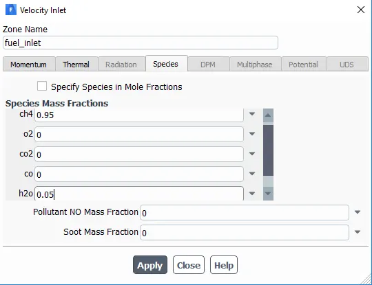
* Under the species tab we can set the mass fraction of fuel and water such that total mass fraction counts 1.
* So in this simulation mass fraction of water is varied from 0.05 all way till 0.3 with increments of 0.05 i.e from 5% of mole fraction to 30% of mole fraction and the formation of soot and `NO_x` at each case are noted. Below are the reusult obtained,
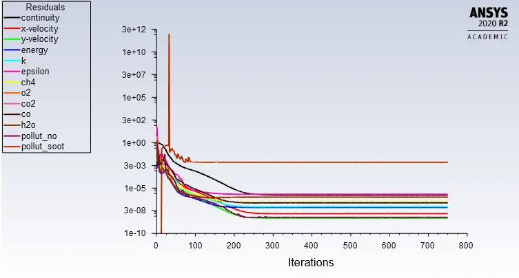
* At 5% of water
* Residual plot:
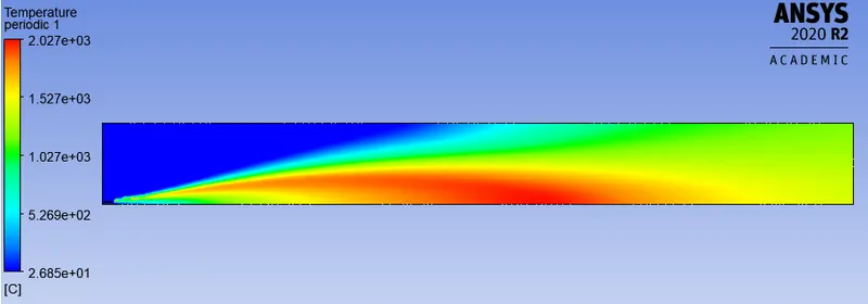
* Temperature contour:
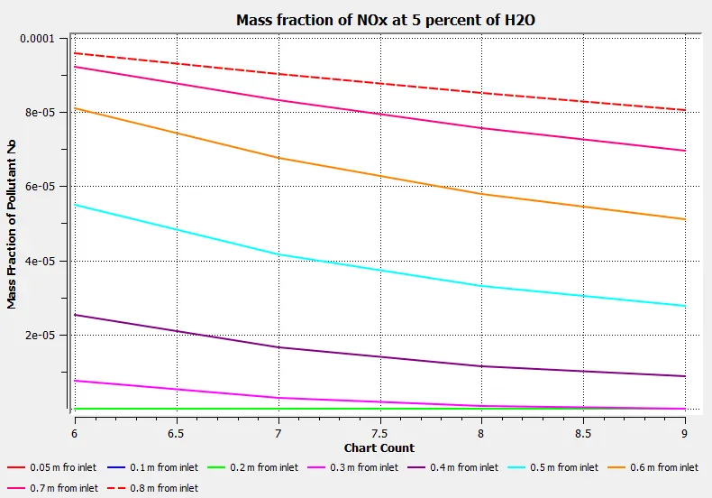
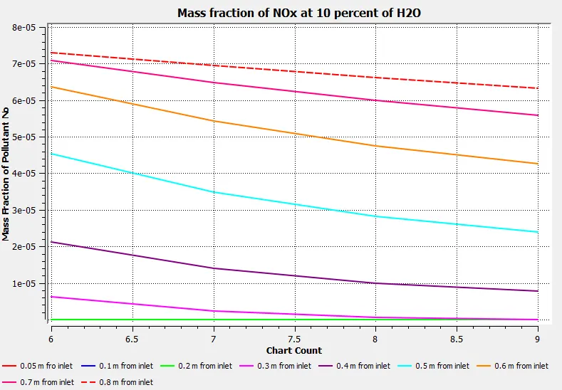
* Mass fraction of `NO_x`:
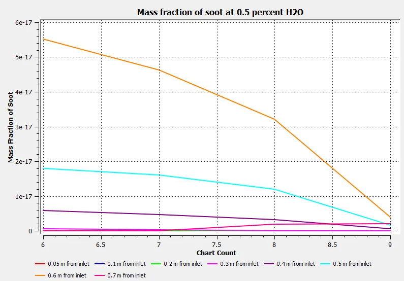
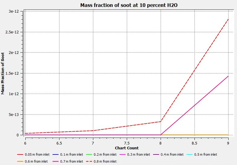
* Mass fraction of soot:
* At 10% of water
* Residual plot:
* Temperature contour:
* Mass fraction of `NO_x`:
* Mass fraction of soot:
* At 15% of water
* Residual plot:
* Temperature contour:
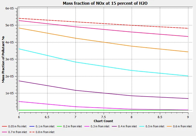
* Mass fraction of `NO_x`:
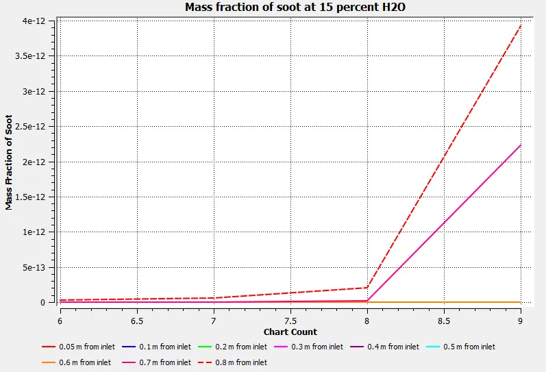
* Mass fraction of soot:
* At 20% of water
* Residual plot:
* Temperature contour:
* Mass fraction of `NO_x`:
* Mass fraction of soot:
* At 20% of water
* Residual plot:
* Temperature contour:
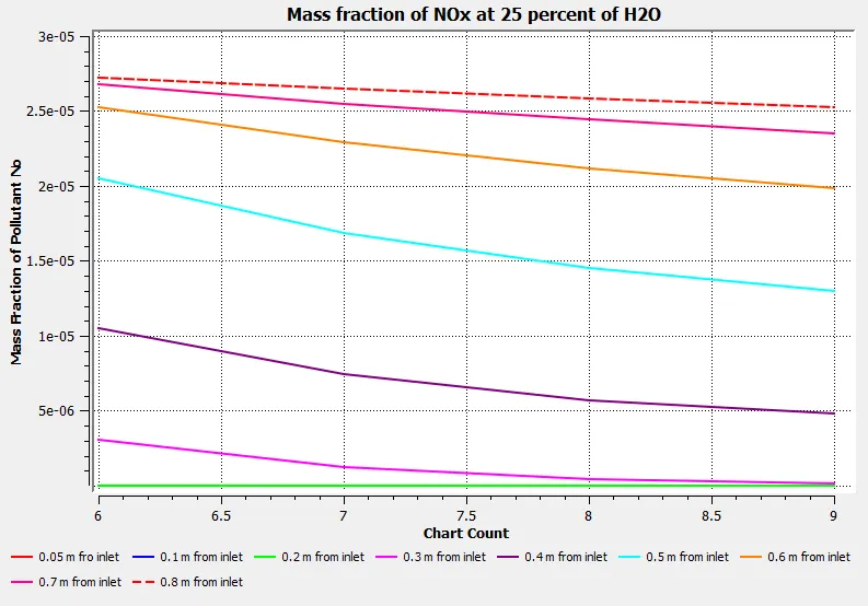
* Mass fraction of `NO_x`:
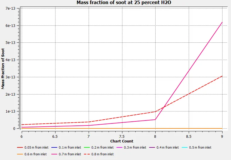
* Mass fraction of soot:
* At 30% of water
* Residual plot:
* Temperature contour:
* Mass fraction of `NO_x`:
* Mass fraction of soot:
Observation:
* As the water content in the fuel is increased the max temperature attained by the combustion process decreases. This can be understood by observing the temperature contour.
* With increase in water content concentration of both `NO_x` and soot at outlet also decreases.