Rayleigh Taylor Instability Challenge
# Aim:
* To study and explain different mathematical models used to study Rayleigh taylor waves and how it is used in CFD calculations.
* Define Atwood number, explain the effect of Atwood number on the instability.
* Perform Rayleigh taylor instability analysis on interface of water and air. Run the simulation for baseline mesh observe the instability.
* Perform instability analysis for the above case for a refined mesh and study the instability.
* Perform instability analysis on interface of water and a user defined fluid.
# Introduction:
Rayleigh taylor instability is the disturbance that occur between the interafce of two fluids of varying densities. One fluid will be of higher density while the other one would be of lower density. Water suspended on top of oil is good example of rayleigh taylor instability, the denser fluid moves down along the direction of gravity and displaces the lighter fluid. The displaced lighter fluid moves upward and hence the complete equillibrium disturbes. Before the actual disturbance start the fluids are in equilibrium and the system has a potential energy as disturbance or instability progresses potential energy also decreases. The instability phenomena that takes place is equivalent to fluid accelarating, lighter fluid accelarating into the denser fluid.
Atwood number is usually used to determine the disturbances in rayleigh taylor instability. Atwood number is defined as ratio of density difference to that of sum of densities.
Atwood Number = `(rho_(h) - rho_(l))/(rho_(h) + rho_(l))`
Rayleigh taylor instability theory says that when Atwood number is close to zero, usually when it is less than 0.5 the instability starts as a parallel symmetric finger like projection of fluids where as when Atwood number is close to one the instability starts looming as bubbles of lighter fluid moving into the denser fluid. These explained disturbance patterns are not predominantly seen but for a range of Atwood number this is how the disturbance starts but as time progresses the disturbance patterns changes completley.
* Different models were deveoped from time to time to study the surface free flows. These models were also effectively used to study the Rayleigh taylor instability as well.
Some of the models and its characteristics is briefly explained below,
1. Marker and cell method:
This is the first method used to model the free surface flow. It is based on a eulerian grid of control volumes. The position of the fluid within the control volumes are determined with theset of marker particles that move with the fluid.
2. Lagrangian method:
In this the grid moves along with the fluid since both grid and fluid moves together the grid automatically follows free surface. Main disadvantage of this method is that it cannot determine the surfaces that intersect or break apart.
3. Volume of fluid method:
It uses a continuity equation for volume of fluid to capture the interface change. In earleir implementation numerical diffusion of interface was a major problem with this model but later on this was eliminated by reconstruction of interface from the volume fraction in computational cells with geometrical elements. Simple line interface calculation (SLIC), flux line segment for advection and interface reconstruction (FLAIR), least square method are used for interface reconstruction.VOF method is used in many commercial cfd codes such as fluent and CFX. The algorithm of VOF method is based on a well defined second order geometric solution of a volume evolution equation. This method utilizes the local discrete material volume and velocity data to track interfaces of arbitraraly complex topology. This ensures that the solution generated maintain second order spatial accuracy. This method was tested to track interfaces through large controlled topology changes.
4. Level set method:
This method uses level set function, which is positive in the space occupied by the first fluid and negative in the space occupied by the second fluid. Level set function is defined as the minimum distance to the interface and interface is defined with zero value of level set function.
# Simulations:
Case 1: Rayleigh taylor instability is observed on water air interface for a base line mesh:
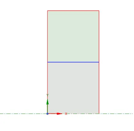
Setup: The simulation carried out is a 2D simulation. Two square surfaces each of dimension 20 mm is created on the x-y plane in spaceclaim. Surfaces are named as air and water, share topology option is used so that the common edge between the two surfaces are shared.
The geometry created looks as follow:
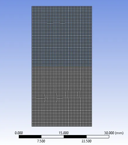
Above geometry is meshed, a base line element thickness of 0.5 mm is initially given and simulations are run. When meshed the above geometry looks as follow,
Solver setup: Pressure based transient solver is used to run the simulations. Since this is a simulation involving multiphase the value of gravity in the negative y direction is also provided. A part from this initial setup the materials are provided from the fluent database, viz air and water. Also multiphase option is selected and in there implicit method is selected also the 2 phases are also defined and are named. Solution contour can be added for the phase change of water so as the animation of the same is added. after this standard initialisation is done Patch needs to be added this is done for volume fraction of water and air, for water a value of 1 is set and for air it is set to 0. Simulations are run for a total of 150 iterations with a time step of 0.005 sec.
* Result:
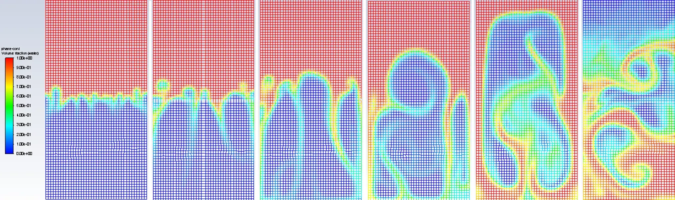
Below are the grab of phase change captured at different time steps,
Video link for the animation of above phase change : https://youtu.be/5vm5saMBDlM
* Case 2: Rayleigh taylor instability is observed on water air interface for a refined mesh:
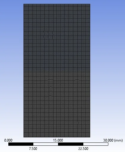
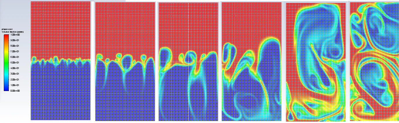
The geometry, solver setup all are same the only change applied is mesh refinement. Element size of 0.25mm is applied and simulations are carried. The refined mesh looks as follow,
* Result:
Below are the grab of phase change captured at different time steps,
Video link for the animation of above phase change : https://youtu.be/Uqyol1BUWEE
*Explaination:
Since both of the above simulations were carried out for the water, air interface let us start with calculating the Atwood number,
Atwood number = `(rho_(h) - rho_(l))/(rho_(h) + rho_(l))`
where `rho_l = 1.225 (kg)/m^3` and `rho_h = 998.2 (kg)/m^3`
therefore Atwood number = (998.2-1.225)/(998.2+1.225) = 0.997
so as per theory for Atwood numer close to 1 the instability or disturbance should start in the form of bubbles of lighter fluid rising, so in the above case for base line mesh of 0.5 mm the bubble formation is visible, but when mesh is refined it is more clear. Moreover the type of disturbance pattern that is observed for base line mesh as well as refined mesh is completley different. Hence we can conclude that as mesh size changes the disturbance patterns observed also changes.
* Case 3: Rayleigh taylor instability at water and user-defined material interface:
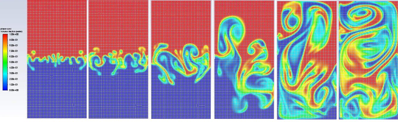
In this case air is replaced by a user defined material of density = 400 kg/m^3, viscosity = 0.001 kg/m-s. Element size of 0.25 mm is used while creating the mesh. Solver setup remains the same.
Below are the grab of phase change at different time step,
Video link for the animation of above phase change : https://youtu.be/3l_tIWrIJpo
If we calculate atwood number for the above simulations we have, atwood number = `(rho_h - rho_l)/(rho_h+rho_l)`
`rho_h = 998.2 (kg)/m^3`
`rho_l = 400 (kg)/m^3`
therefore, Atwood number = (998.2-400)/(998.2+400) = 0.4
so as per the rayleigh taylor instability theory for Atwood number close to zero the disturbances starts as symmetric finger like projections of the lighter fluid and then disturbance grows. when water and air interface instability is observed the disturbances started like bubbles but here it is more of a finger like projection. Also the mesh refinement helped in capturing the effect of disturbance quite well.
#Steady state simulation of Rayleigh taylor instability: This is not a good option to study the instability because rayleigh taylor instability is observed more as accelaration of fluid, i.e accelaration of lighter fluid into the denser fluid and hence causing the disturbance. Accelaration being rate of change velocity w.r.t time, it is more of transient nature than that of a steady state hence if we carry out the steady state simulation of Rayleigh taylor instability it wont be possible for us to observe the phase change as well as the disturbance that continues.
Below is the snip of the phase change contour for a steady state simulation for instability carried on water-air interface,
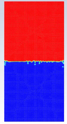
It is clearly observed that small disturbance can be seen in the interface but the whole phase change cannot be obtained.