Week-11 : Discretization of 3D intake manifold using GEM-3D
AIM
* To run simulation on single cylinder DI engine for 2 cases, first one with default case and second one with discretization length of 0.1 mm for intake runner and compare the result using parameters such as torque, bsfc, max cylinder pressure.
* To explore tutorial number 2 and to build a intake manifold from STL file using GEM3D.
INTRODUCTION
Discretization being the main focus of this assignment it will be better if we understand what discretization is and what is its purpose. Discretization is nothing but dividing any fluid volume into smaller sub volumes of equal length or different length. Flow parameters such as pressure, temperature, mass fractions etc are calculated in each sub volumes. In a simulation if explicit solver is used then the time step required is directly proportional to the discretization length. Smaller the discretization length more number of sub volumes will be formed and hence solver will take more time to solve. The proportinality between the time step and discretization length when a explicit solver is used is as shown below,
`Deltat_e prop (Deltax)/(c + abs(u))`
`Deltat_e -` Explicit time step
`Deltax -` Discretization length
`c -` Speed of sound
`u -` Flow velocity
GT-suite provide certain recommendations regarding on setting discretization length for different simulation scenario. For engine simulations (explicit solver) the discretization length of intake system can be set to 0.4 time the bore where as for exhaust system the discretization length can be set to 0.55 time the bore. Difference in the discretization length for intake system as well as exhaust system comes form the point that the speed of sound is temperature dependent. Discretization length should be decreased for acoustic simulation as well as engine performance simulation at engine speed more than 6000 rpm.
Liquid system simulation which uses implict solver in such simulation a discretization length of 40-50 mm can be used. Simulation of cooling system and lubricating system uses implicit solver and also capturing the wave dynamics is not that important and hence larger discretization length can be used. When liquid systems are modeled using explicit method then discretization length of 10-20 mm can be used.
* Single cylinder DI engine:
This is a tutorial case in GT-suite, the path of the same is Tutorials/Modeling_Applications/Engine_Performance/1cylDI
The project map is as shown below and followed by this a brief explaination of the model is given,
* Starts from an endenvironment env-inlet-1 where the boundary condition are set, temperature of air is set at 300 K with a pressure of 1 bar and the fluid composition is set to air.
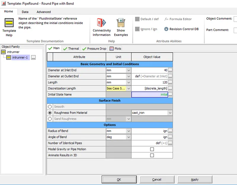
* Next is intake runner which is modeled using a template, inlet and outlet diameter is set to 40 mm with a length of 120 mm. Discretization length is set to 40 mm, this is the default discretization length since the target is to check the affect of discretization length on different performance parameters this attribute is set as a case parameter.
* Initial state of the fluid inside the intake runner is set same as that in the end environment. Cast iron is the material set for intake runner.
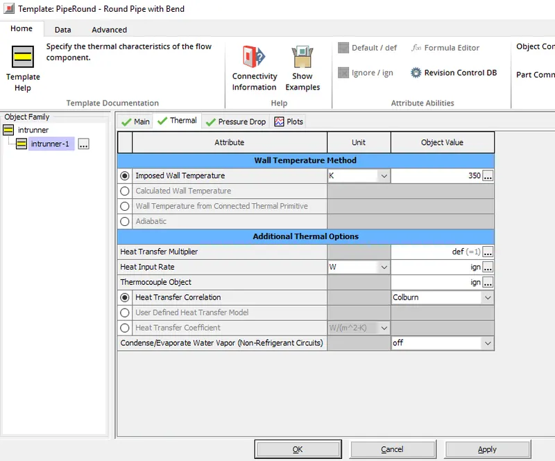
* In thermal folder the imposed wall temperature is set to 350 K and the heat transfer corelation is set to colburn. Pressure drop in intake runner is not considered and hence attributes in the pressure folder is ignored. A snip of attributes set under each folder is shown below,
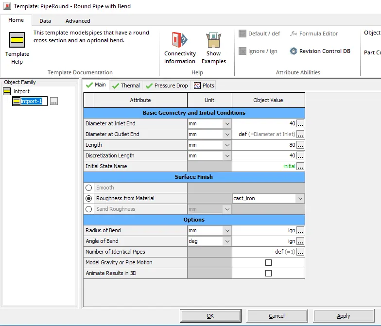
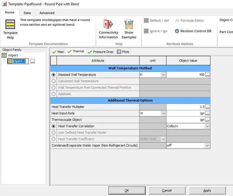
* Flow next takes place through intake port, with inlet and outlet diameter of 40 mm. length of 80 mm and discretization length of 40 mm. Material of the intake port is set to cast iron. In thermal folder the imposed wall temperature is set to 450 K and heat transfer corelation is set to colburn. A snip of the same is provided below,
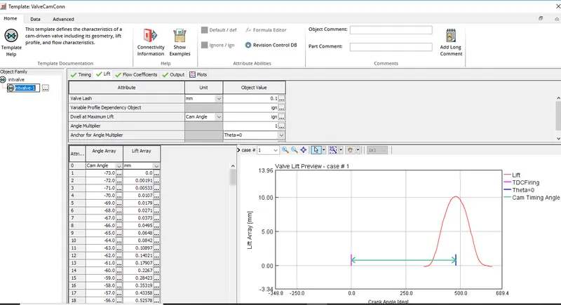
* Flow of air into the combustion chamber is metered using a intake valve. Valve lift profile is set with reference to cam angle. Below is the snip of valve lift profile,
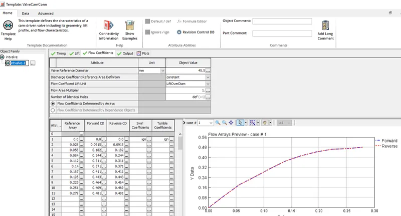
* Setting up the flow coefficients is as important as setting up the valve lift profile, a snipof the flow coefficients set is as shown below,
* After setting different attributes pretaining to intake valve next comes defining certain combustion modeling related attributes. First attribute among defining combustion modeling is setting the initial state of air as it enters the cylinder, tempaerature is set to 350 K and a pressure of 2.4 bar is set.
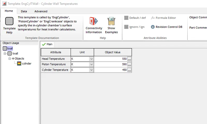
* Head temperature, piston temperature and cylinder temperature is set as shown below,
* In cylinder heat transfer is modeled using the WoschniGT model, head to bore area ratio is set to 1 and piston to bore area ratio is set to 1.2.
* Next important attribute is defining the combustion model. Since the purpose of this simulation is to study the affect of intake runner discretization length on certain performance parameter, a non-predictive combustion model is very much fine. DI-wiebe combustion model is set, since this is a non-predictive combustion model the fuel burn rate is imposed by the user. Fuel burn rate is set by defining the fraction of fuel burned in premixed fraction, tail fraction, respective durations. A snip of the same is shown below,
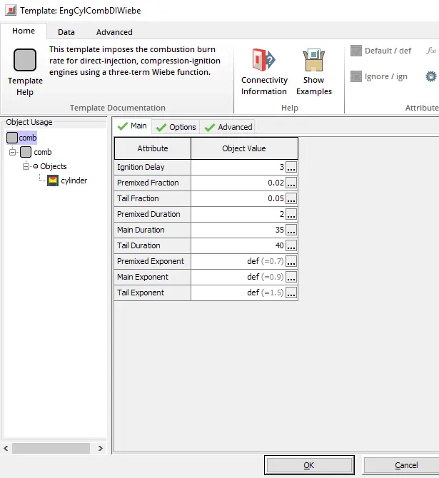
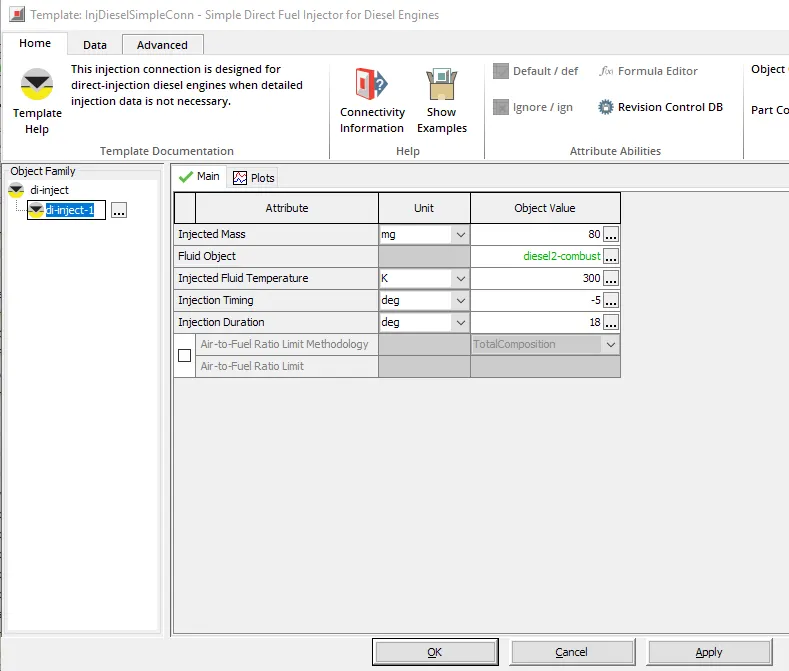
* Since this is a diesel engine the injector that injects fuel into the combustion chamber is to be modeled. A injector template is used, where the mass of fuel injected per cycle is set to 80 mg. The fluid that is being injected needs to be set, diesel-2 combust is the fuel type set and this fluid reference object can be found in GT-suite library. Injected fluid temperature is set to 300 K. Start of injection is set at -5 degree of crank angle (i.e 5 degree before TDC) also the duration of injection is set to 18 degree.
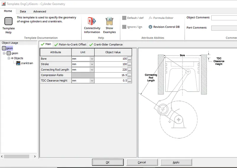
* Cylinder geometry of the engine is as shown below,
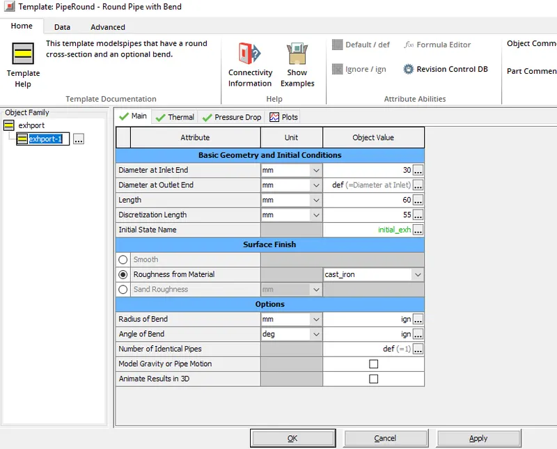
* On the exit side we have a exhaust valve through which the exhaust gases are vented out. Valve lift profile as well as the flow coefficients defined are same as that of intake valve. Through exhaust port the exhaust gases flow into exhaust port. Inlet and outlet diameter of the exhaust port is set to 30 mm, with a length of 60 mm and discretization length set at 55 mm, initial state of exhaust gas in the exhaust port is set at 1.1 bar pressure and temperature of 750 K. Cast iron is the material set for the exhaust por.
* In thermal folder the imposed wall temperature is set to 550 K and the heat transfer corelation is set as colburn. Snips of the above discussed attributes are shown below,
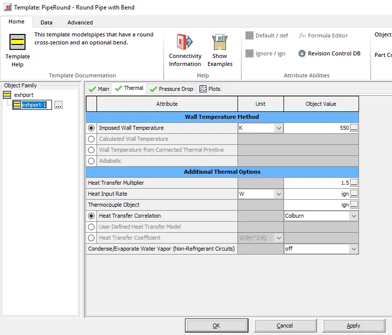
* After exhaust port there comes exhaust runnere, inlet and outlet diameter of the exhaust runner is set to 30 mm, length is set to 150 mm and discretization length is set as 55, initial state of exhaust gases inside the exhaust runner is set to same initial conditions as that of exhaust port. Steel is the material set for the exhaust port. In thermal folder the imposed wall temperature is set to 600 K and heat transfer corelation is set to colburn.
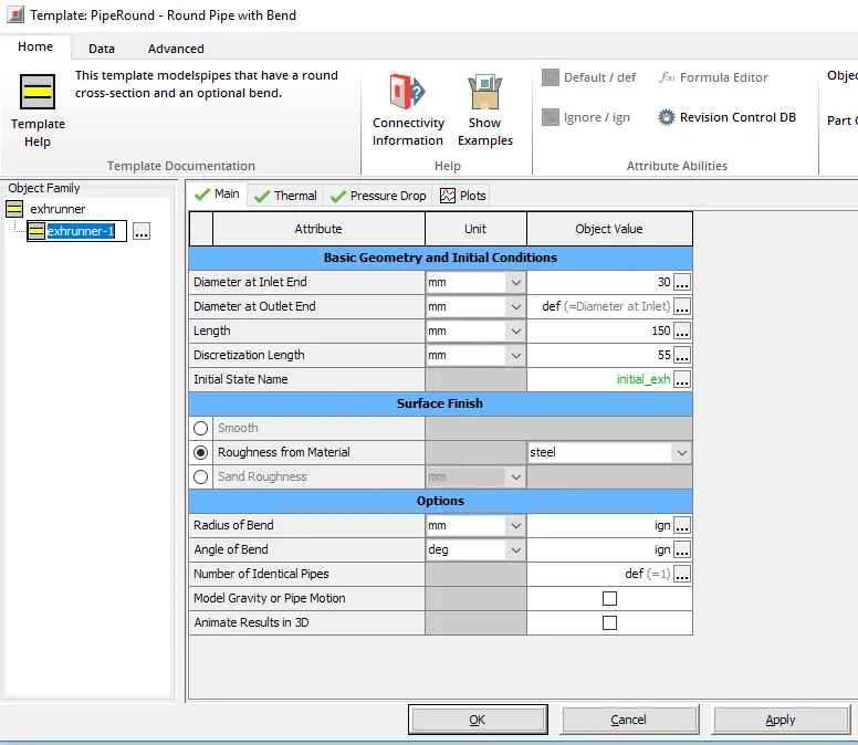
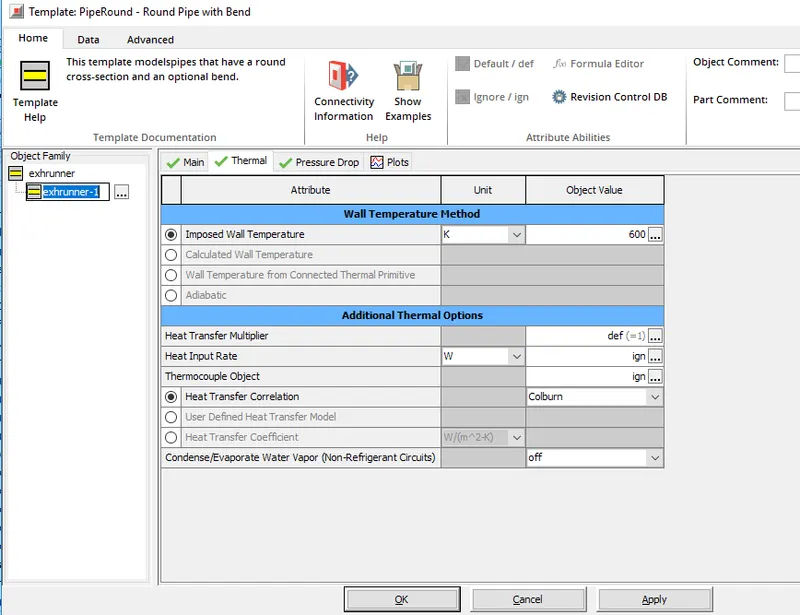
* Default discretization length of intake runner is 40 mm, since discretizaton length is set as a parameter, one more case is being added where the discretization length is set to 0.1 mm. A snip of the case setup window is shown below,
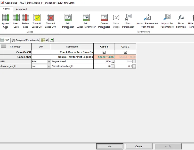
With above shown parameters the simulation is run and results are noted.
* Result and observation:
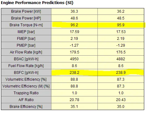
* Torque gets decreased and bsfc is increased, and time taken for case 2 to converge is more, since the discretization length is set to 0.1 mm, 120/0.1 = 1200 sub-volumes are created in each subvolume the flow parameters needs to be calculated and hence case 2 is more time consuming.
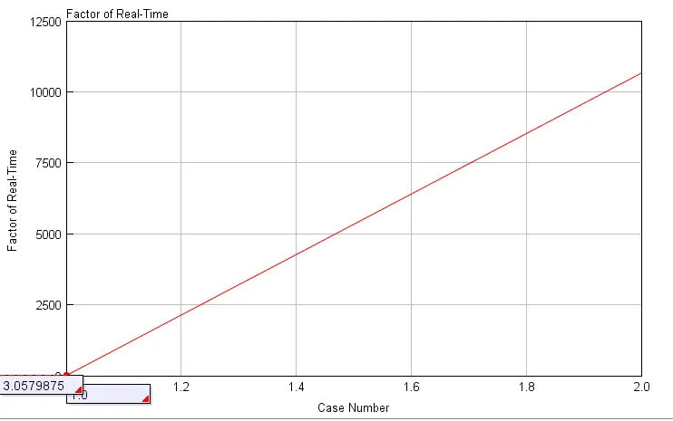
* Below plot of real time factor v/s case gives a clear picture how simulation time has increased drastically as we move from case1 to case2
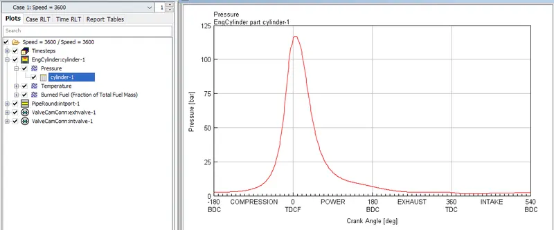
* As far as the incylinder pressure is concerned, snips of the same at case 1 and case 2 is shown below,
case1 incyinder pressure:
case2 incylinder pressure:
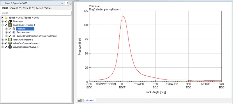
From the above plots it is concluded that discretization length of intake runner doesnt effect incylinder pressure as such.
* To build a intake manifold using GEM3D:
Intake plenum through which intake charge enters the cylinder, STL file of the plenum geometry is opened in GEM 3D tool, plenum geometry is opened as a surface file. A snip of the same is shown below,
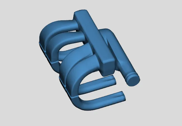
* Under convert option, there is a tool using which we can separate the geometry using curves. When this is used we get the geometry as shown below,
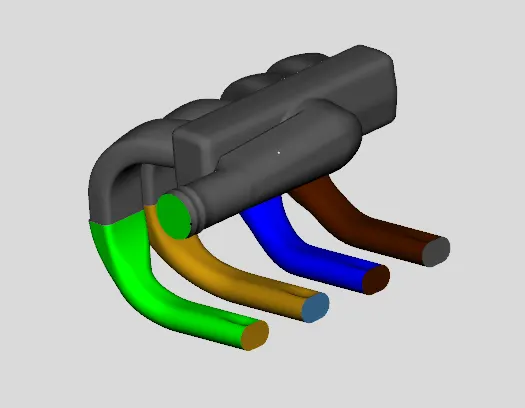
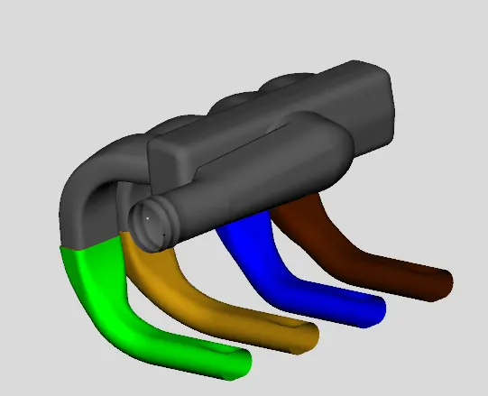
From the above the fluid entry openings are deleted,
* Next step is to split the port on the intake side, to achieve this we can use a 3 point cutting plane (this is a option available in convert). Three points are clicked on the plane parallel to which the cutting plane needs to be formed. A snip of the cutting plane formed is shown below,
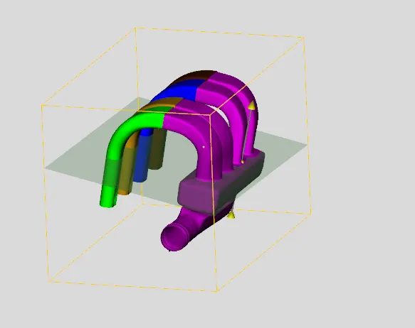
* When splitted it looks as follow,
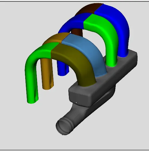
* All the intake runners have multi bend and hence it is must that we convert it into one with circular cross-section. By right clickng anyone of the runner we will get an option called convert shape to component, we get a window as shown below,
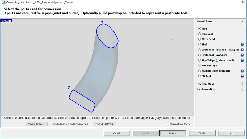
* There are several options present, we can convert the multibend intake runner into a pipe, flow split, miter bend etc, here we go with pipe. By clicking next a window appears as shown below,
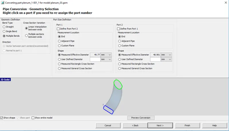
* With the help of different attributes in this window we can set the diameter of the circular pipe. We can use the custom plane to set the diameter. Diameter of 48.6 mm is set for port 1 and same is being used in port 2 using the define from port1 option.
* Clicking next takes us to another window as shown below which has folders such as Geometry, XYZpoints, cross Sections, Location, Flexible Wall. A snip of the same is shown below,
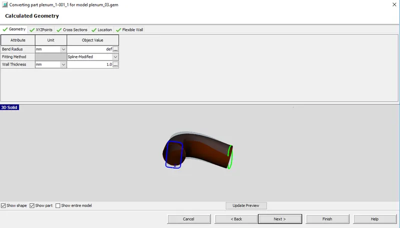
* Wall thickness is set to 1, XYZ points folder has the X, Y, Z co-ordinates of 65 points in the geometry these are the points that define the geometry. In cross-sections folder the length of the pipe and diameters are defined. A snip of the XYZ points window as well as the cross-section is shown below,
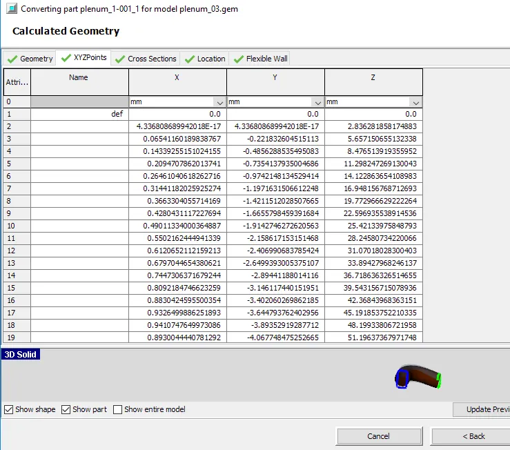
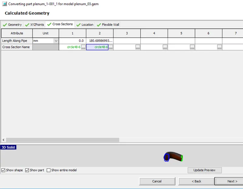
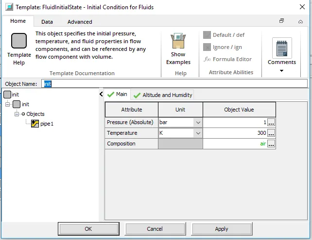
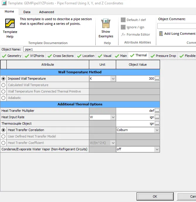
* Initial state of the fluid inside the runner is set to 300 K temperature, 1 bar pressure and fluid composition is set as air. In thermal folder the imposed wall temperature is set to 300 K and heat transfer corelation is set to colburn.
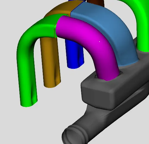
* Once we complete till above disscussed points the intake runner with multiple bends gets converted into one with circular cross-section. A snip of the same is shown below,
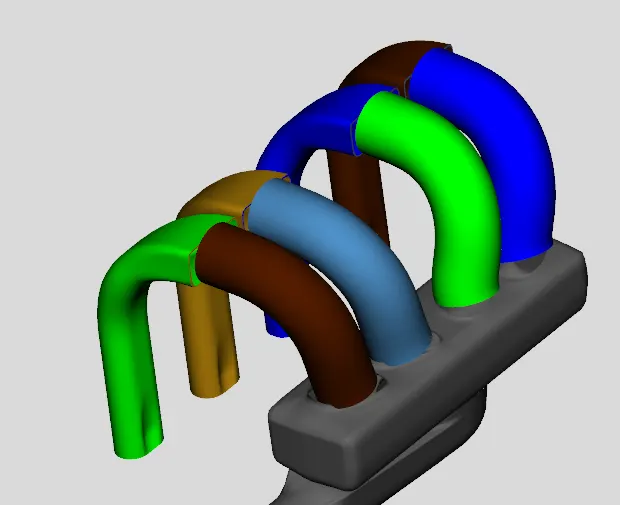
* We can convert the other intake runners into one with circular cross-section, same above mentioned steps are followed and each intake runners are converted manually. When all the intake runners are converted into one with circular cross-section, we have as shown below,
* Like intake runners the intake port needs to be converted circular cross-section, same above mentioned steps are being follwed and it is converted into one with circular shape.
* One of the intake port is selected, in the further window where the diameters at port1 and port2 is defined, for port1 a diameter value of 51.6 mm and for port2 a diameter value of 38.3 is defined, since there is a drastic change in shape as we progress from port1 towards port2 two different values of diameter is set.
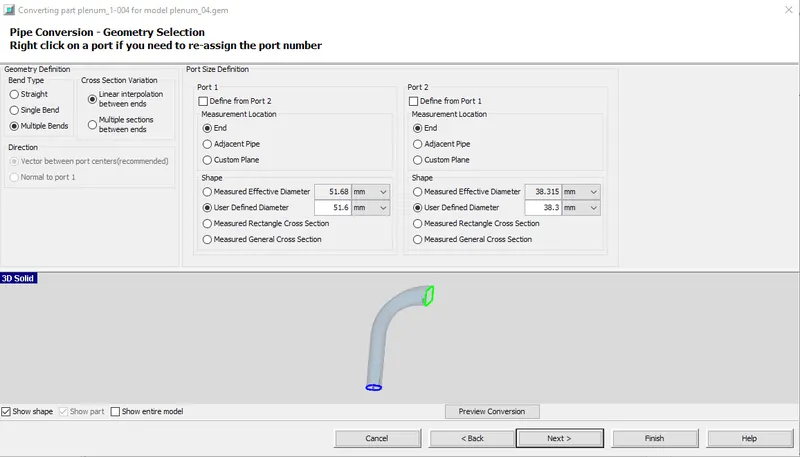
* Other parameters pretaining to initial conditions such as temperature, pressure and composition as well as the imposed wall temperature, heat transfer corelation gets automatically set to the value defined previously for intake runners. The converted intake port looks as follow,
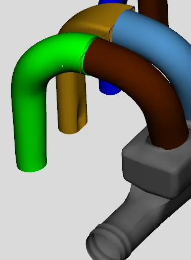
* Similarly all other intake ports are converted into circular shapes, snip of the same is shown below.
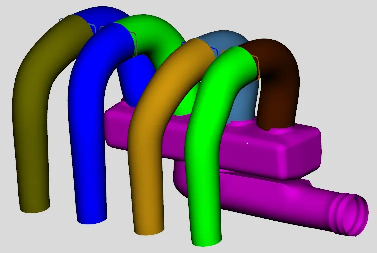
* Coming back to intake runners since it is a geometry with circular cross-section the entry of fluid from the plenum into the intake runner should have smoothly. To achieve this the forward discharge coefficient needs to be set. By right clicking on any of the intake runners we will get option to add flow connections.First when it is selected we get something shown in below snip.
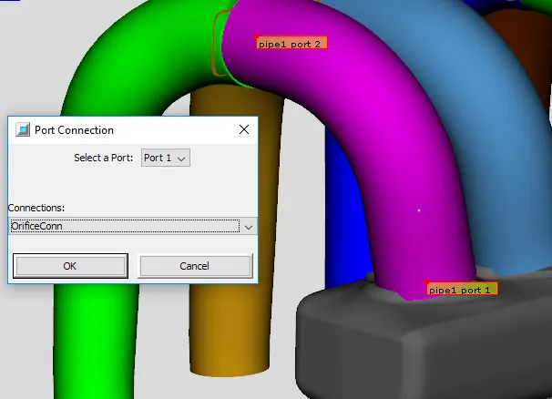
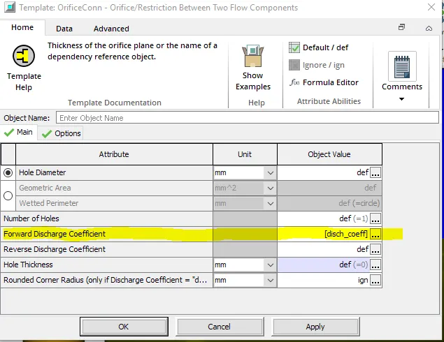
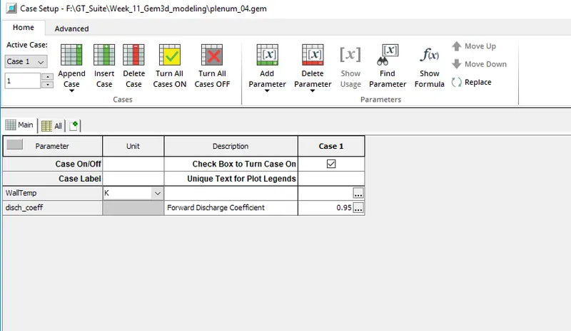
* Tool asks for the location where the flow connection to be added, since we are interested at intake runner-plennum intersection we can select port1. From the drop down menu we can select the type of connection to be added in here the orificeConn is selected. By clicking ok another window opens where there are number of parameters pretaining to setting up a orifice connection. In this window the attribute forward discharge coefficient is set as a parameter and in the case setup a value of 0.95 is defined. Snips of the orifice conn setting up window as well as case setup window are shown below.
* In same way the forward discharge coefficients for other runners are set. Next step is assigning the exit of intake ports with the outlet id, so as to do this we have to right click on any on eof the intake port from the menu we get we can select add connection. It asks for the port number where the outlet id to be added, for all the intake ports this is port2 after that from the drop down menu we have to select the type of connection, GEMSubAssExtConn and ok is clicked. On clicking ok we get another window where the port id and type of boundary is defined.
* Next comes conversion of plenum as pipes and flow splits. By opening the convert tab in the tool bar we get following options to select.

from this the pipe normal cutting plane tool is selected. We can click anywhere in the plenum to get the pipe normal cutting plane. Below snip shows the cutting plane along with the plot that automatically pops up as we click.
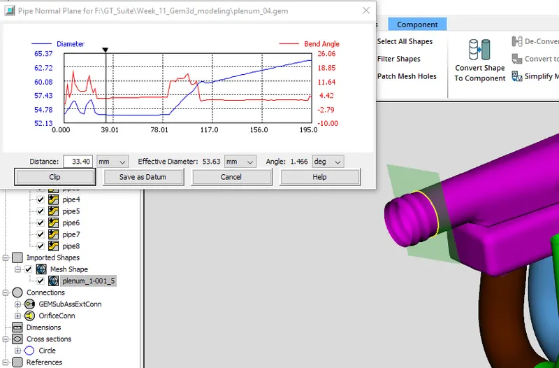
* In the plot we can see the diameter and bend angle plotted against the length. We can select a diameter where there is no abrupt variations in diameter as well as bend angle. When splitted using a normal plane we get a pipe as shown below,
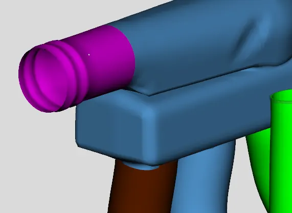
* Another half of the plenum is also splitted in the same way as above. A snip of the same is shown below,
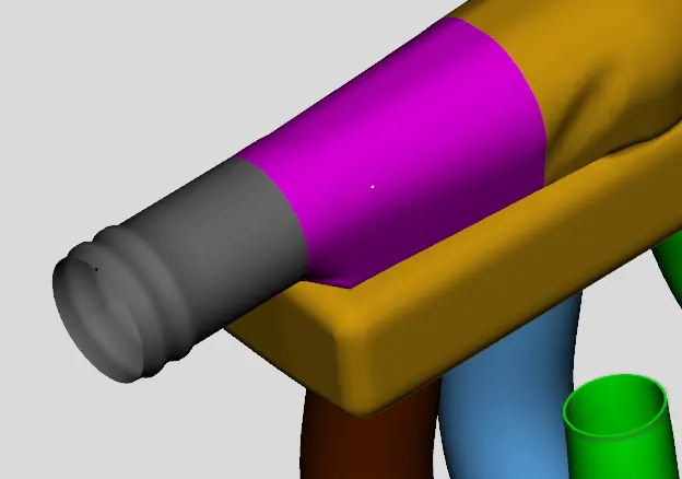
* Two parts created from intake plenum is converted into circular shapes. Steps followed in converting these into circular ones is the same as followed while shape converting the intake runners and intake ports. Starting from the first pipe we have,
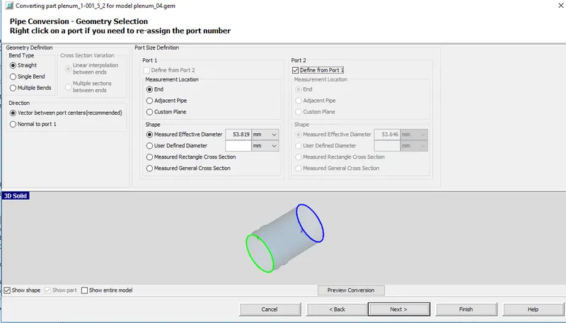
* Instead of converting it into a pipe with multiple bends it is converted into a straight pipe. Diameter at port2 is defined to fetch from port1, apart from this the initial condition and imposed wall temperature gets automatically defined to the one which is defined for intake runners, intake ports. When converted we get a straight circular pipe as shown below,
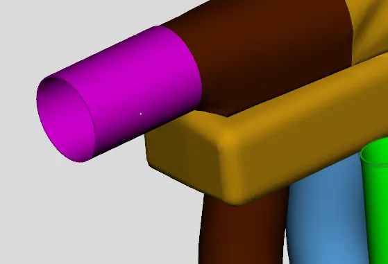
* Next part is the one with the step, even this is converted into a straight circular pipe.
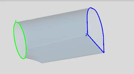
Since this part has a larger diameter at port2 the same can be used as the diameter of the pipe and hence the diameter at port1 is fetched from port2. Initial condition and imposed wall temperature remains the same. When converted we get a circular pipe as shown below,
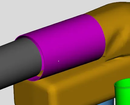
* port1 of the intake pipe is set as an inlet using the add connection option.
* When all the converted parts are hidden we get something as shown below,
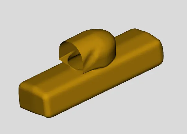
* The above shown part of the plenum is splitted and converted into pipes or flow splits accordingly. After splitting we get two parts, one as shown below
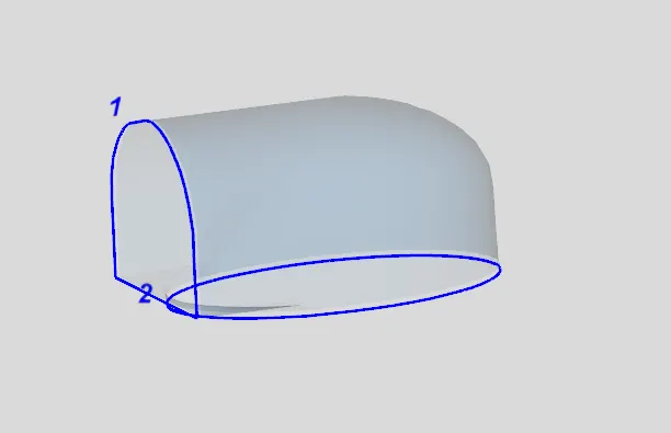
* This being a 90 degree flow angle rather than converting this shape into a pipe it will be better if we convert this into a flow split. Conversion to flow split doesnt ask for the diameter value at port1 and port2, a general type of conversion forms a boundary data as shown below, apart from this the initial conditions and imposed wall temperature remains the same.
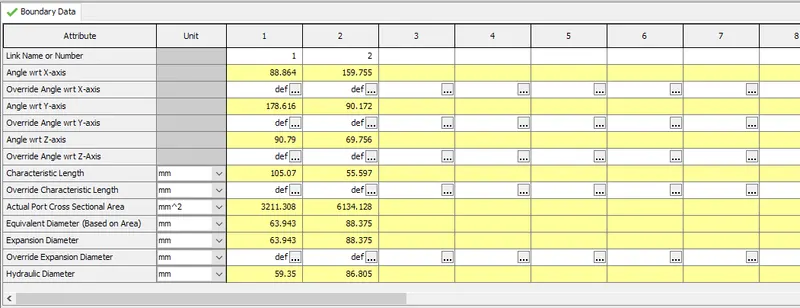
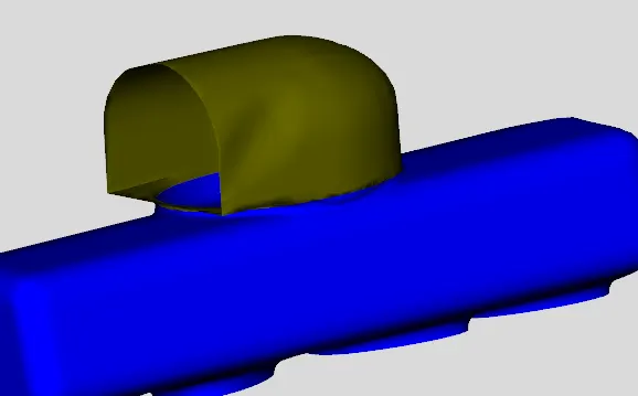
When converted into a flow split we get the converted shape as,
* Now the only part remaining to be converted is,
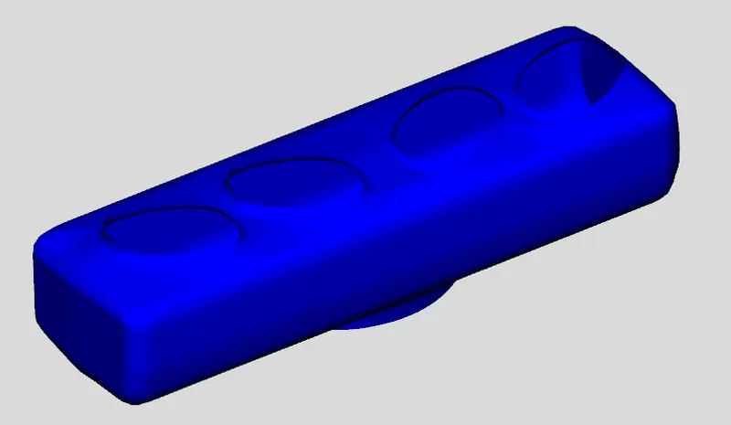
To split this again the 3 point cutting plane is used, the part is splitted into three using a plane which is perpendicular to the part.
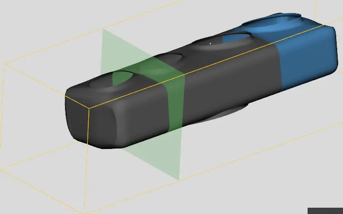
* When splitted we get a shape as shown below,
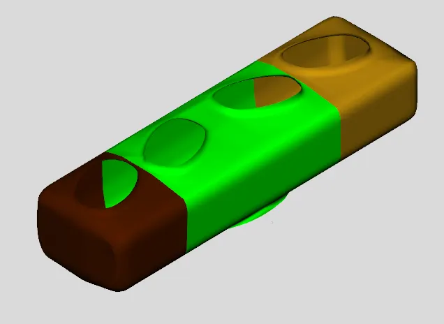
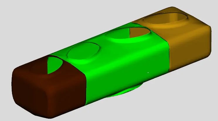
* Now the three split shapes are converted into flow splits. Same method as mentioned in the above conversion is used along with same initial conditions and imposed wall temperature. When converted we get the entire shape as flow splits as shown below,
* Next step is to take care of gaps, because of conversion of shape into specific components many gaps are generated which needs to filled. Flow connections and extrude cpnnection options can be used to achieve the same. Snips of the gaps present in the component is shown below,
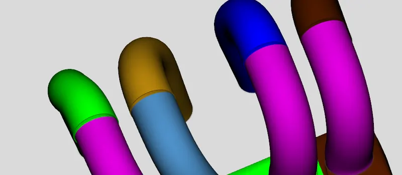
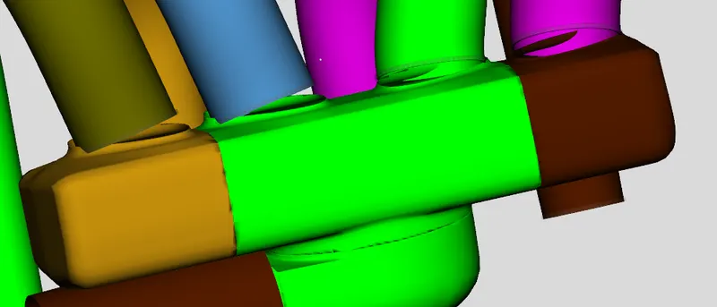
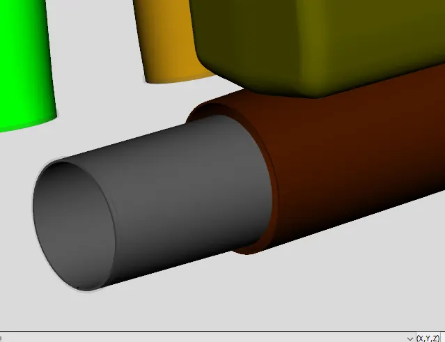
By using flow connections we get many planes at different gaps where possible flow connections can be established. A snip of the planes generated is shown below,
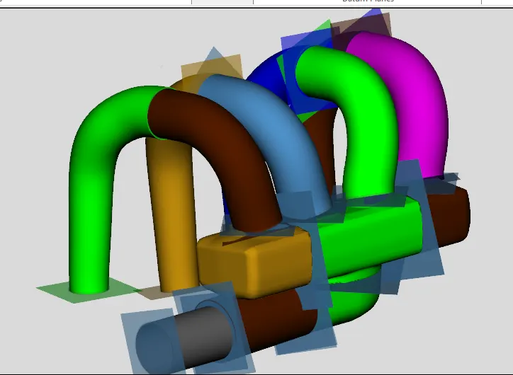
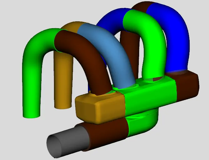
By selecting the two planes possible flow connections can be established, When the flow connections and extrusions are complete we get the complete component as shown below,
The component so created should be oriented properly before it is exported into a GT-ISE model, by selecting the export to GT-ISE model a window appears which has the discretization length, shell discretization length along x, y, z direction. Snip of the same is shown below,
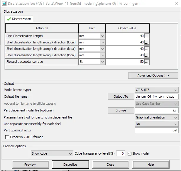
when exported into GT-ISE we get the the complete component as shown below,
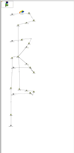
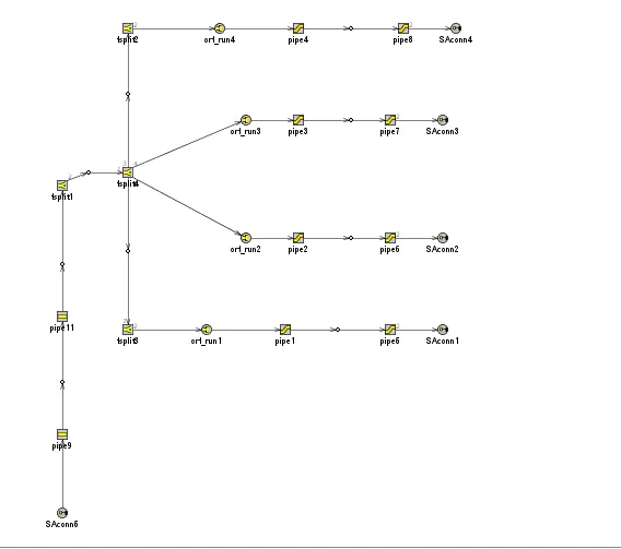
Above can be arranged in a well manner and a project map as shown below can be obtained.