Week 9 - Mini project - Flow over an Airfoil
AIM
* To create a NACA 2412 airfoil using the coordinates available.
* To run an external aerodynamics simulation for different angles of attack.
* To plot the coefficient of lift and drag at different angles of attack.
INTRODUCTION
Lift and drag coefficients are of great importance when it comes to flight dynamics. Different experiments are conducted over different airfoils to study the effect of shape of an airfoil on the coefficient of drag and lift. The aim of these experiments was to reduce the coefficient of drag and increase coefficient of lift for different airfoils. NACA 2412 is an airfoil on which experiments were conducted by NASA.
Before diving into the simulations it will be better if we understand how the flow over an airfoil causes the lift. If we consider symmetricity then there are 2 kinds of airfoils, symmetric airfoils and non-symmetric airfoils. For symmetric airfoils at zero angle of attack (Angle between the flow lines and the chord length) there is no lift generated, for non-symmetric airfoils at zero angle of attack there will be a small lift generated because of the curvature at the leading edge of the airfoil.
When we provide a angle of attack for the airfoil the front stagnation points moves below the leading edge and the trailing edge stagnation point moves to the top surface, this causes the fluid in the bottom surface of the airfoil to separate which forces the stagnation point of the surface to move to the trailing edge and this generates a clockwise movement for the airfoil, which is nothing but a lift.
In this simulation a NACA 2412 airfoil is created in converge-studio and a 2D simulation is run for different angle of attack and from the results obtained the coefficients of drag and lift are plotted against the angle of attack.
The NACA 2412 airfoil profile looks as shown below,
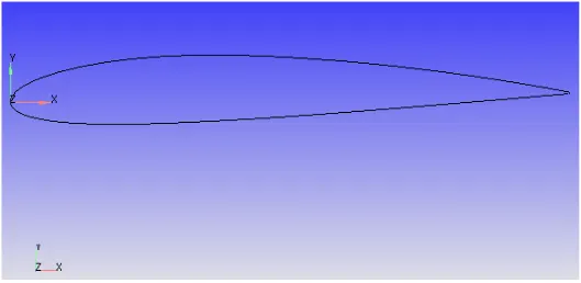
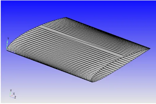
The chord length of the airfoil is 0.1 meter .
The length from leading edge of airfoil to the inlet is set to 0.9 meters, length from trailing edge of the airfoil to the outlet is set to 1.5 meter.
Total height of the virtual wind tunnel is set to 1.25 meter.
Since this is a 2D simulation the length of the wind tunnel along z-direction is not of much importance and hence any appropriate length can be given.
After creating the virtual wind tunnel the geometry is as shown below,
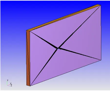
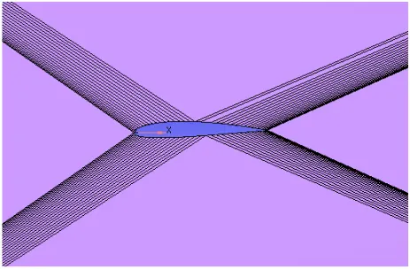
In above shown pictures the angle of attack of the airfoil is zero.
CASE SETUP
* The application type is set as gas simulation with default values of global transport parameters, `O_2` and `N_2` are set as species.
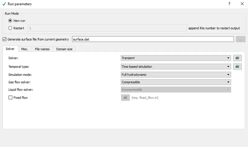
* Under run parameter, a transient and compressible flow with full hydrodynamic simulation is set. Apart from this all other local controls under run parameters are set to default values.
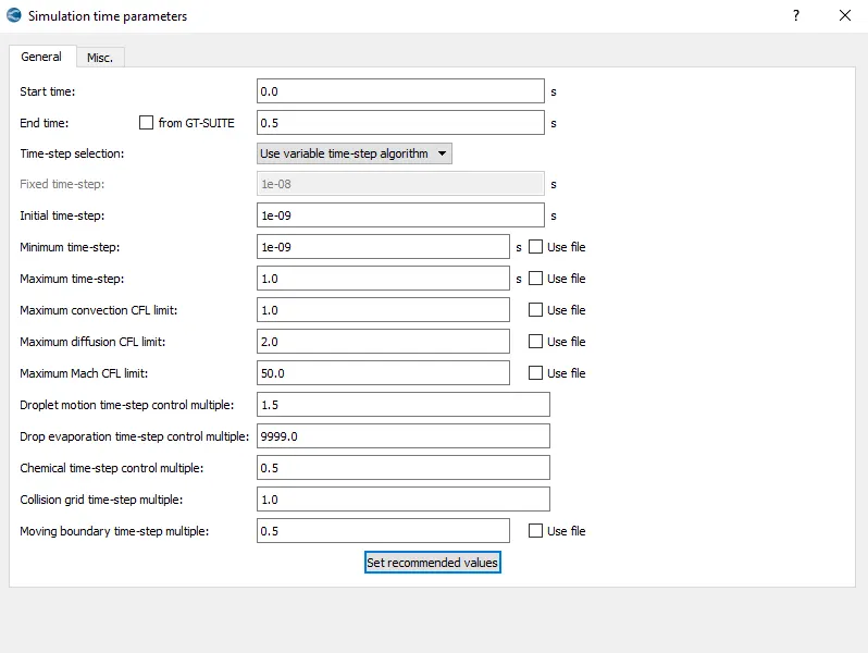
* The start time and end time for the simulation is set to 0 and 0.5 sec respectivley. Initial time step is set to 1e-09 sec, minimum time step is set to 1e-09 sec and max time step is set to 1 sec. Apart from this other local controls under the simulation time parameters are set to default values.
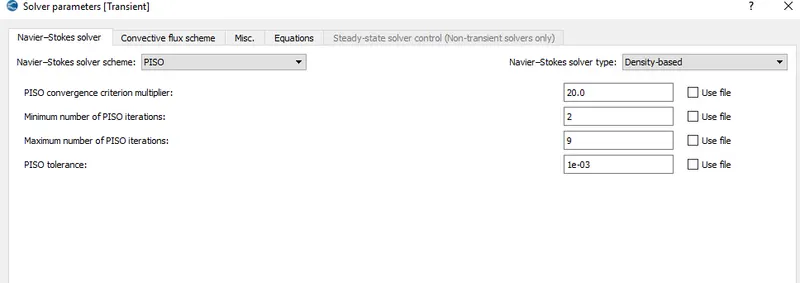
* Under solver parameter the solver type is set to density solver, since the flow is compressible. All other local controls under this solver parameter are set to default values.
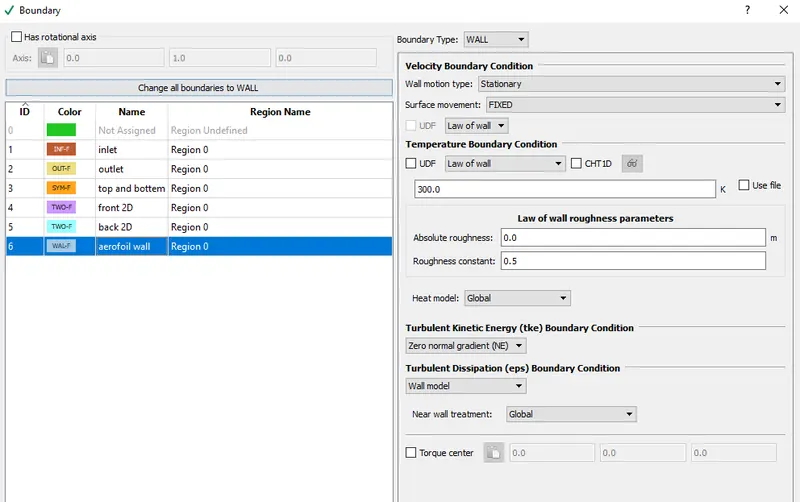
* Next comes defining the boundary condition, total 6 boundary's are defined which are discussed below:
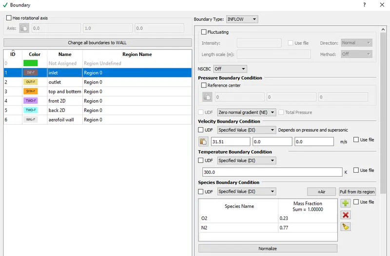
1. Inlet: For this the boundary type is set to inflow. The inlet velocity is specified as 31.51 m/s, which is calculated from provided Reynolds number = 200000. Temperature of the air enetering through the inlet is set to 300 K, `O_2`and `N_2` are set as the spcies.
Reynolds number, `Re = (u*L*rho)/mu`
`rho_(air) = 1.1765 (kg)/m^3`
`mu_(air) = 1.8538*10^(-5) (kg)/(m*s)`
Characteristic length, L = 0.1 meter
therefore Inlet velocity, `u = (200000*1.8538*10^(-5))/(0.1*1.1765) = 31.51 m/s`
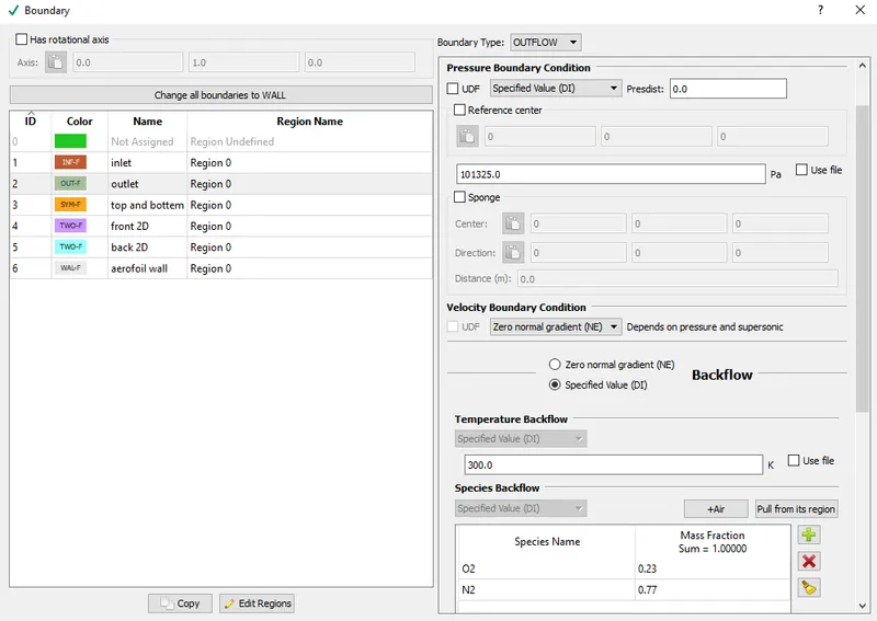
2. Outlet: For this boundary the boundary type is set as outflow. Atmospheric pressure at the outlet is specified, with a temperature of 300 K and `O_2` and `N_2` are set as the species.
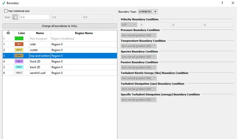
3. Top and bottom: This is the top and bottom walls of the virtual wind tunnel. The boundary type is set as symmetry.
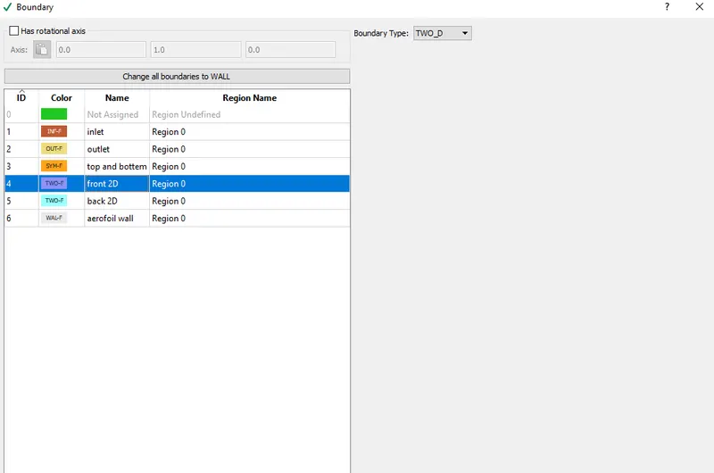
4. Front 2D: This is the front surface, since this is a 2D simulation for this boundary the boundary type is set as 2D.
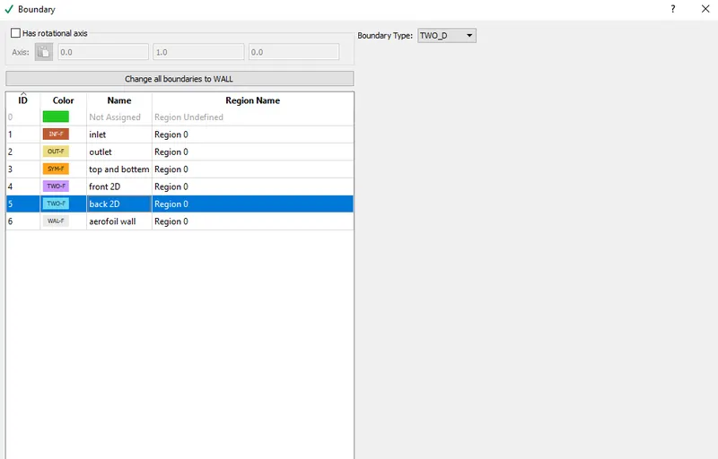
5.Back 2D: This the back surface of the virtual wind tunnel, since this is a 2D simulation for this boundary the boundary type is set as 2D.
6. Aifoil wall: This is the complete airfoil surface, for which the boundary type is set to wall. A stationary wall with law-of-wall boundary condition is applied. Temperature at airfoil is set to 300 K.
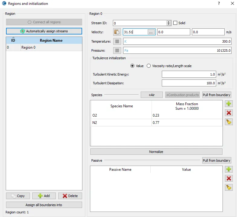
* Next a region is defined with initial velocity of 31.51 m/s and pressure of 101325 Pa, 300 K temperature and this region is labelled as region_0 and all the boundary's defined above are assigned to this region.
* RNG K-`epsilon` is set as the turbullence model to capture the turbullence in the flow. Inflation layers are applied on the airfoil using embedding.
Since K-`epsilon` is the tubullence model used we can use y+ value ranging from 35 and above. First layer thickness calculation is shown below,
`y+ = (rho*u_(tau)*y)/mu`
so from the above we can wirte, `y = (mu*(y+))/(rho*u_(tau))`
where, y is the first layer thickness
`u_(tau) = sqrt(tau_(w)/rho)`
`tau_(w)` - Wall shear stress (N/m^2)
wall shear stress , `tau_(w) = 1/2*C_(f)*rho*V^2`
where, `C_(f)` - Skin friction
Skin friction, `C_(f) = 0.058*Re^-0.2`
`rho_(air) = 1.1765 (kg)/m^3`
`mu_(air) = 1.8538*10^(-5) (kg)/(m*s)`
Velocity of air at inlet, u = 31.51 m/s
Characteristic length (Chord length) of airfoil, L = 0.1 meter
Reynolds number, Re = 200000 (provided)
Skin friction, `C_(f) = 0.058*(2*10^(5))^(-0.2) = 0.0050`
Wall shear stress, `tau_(w) = 1/2*0.0050*1.1765*31.51^(2) = 2.9203 N/(m)^2`
`U_(tau) = sqrt((2.920)/(1.1765)) = 1.575`
Since k-`epsilon` turbullence model is used y+ = 130 is used for first layer thickness calculations,
`herefore, First layer thickness, `Y = (1.8538*10^(-5) *130)/(1.1765*1.575) = 1.30 mm`
* Inflation layers are added using the embedd local control under the grid sizing option. In embedd layering the first layer thickness is calculated using the embedd level defined and the base grid size.
Grid size = Base grid / `2^n`
n - Embedd level
from our calculations we have first layer thckness, y = 1.30 mm
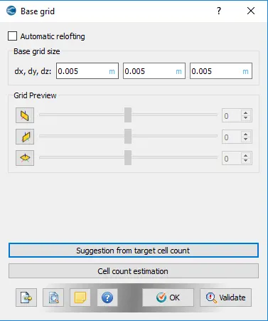
The base grid size is set to 8 mm
therefore, 1.30 = 8/`2^n`
calculating n from the above we get, n = 2.62
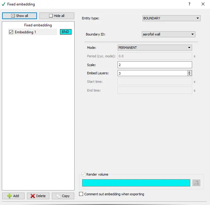
In converge we cannot mention the decimal number as embedd level and hence the embedd level is defined as 2, also a total of 3 embedd layers are defined. This completes applying the inflation layers or body fitted mesh around airfoil.
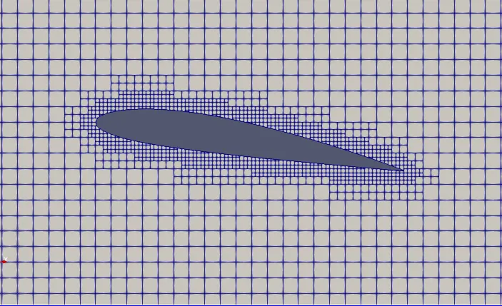
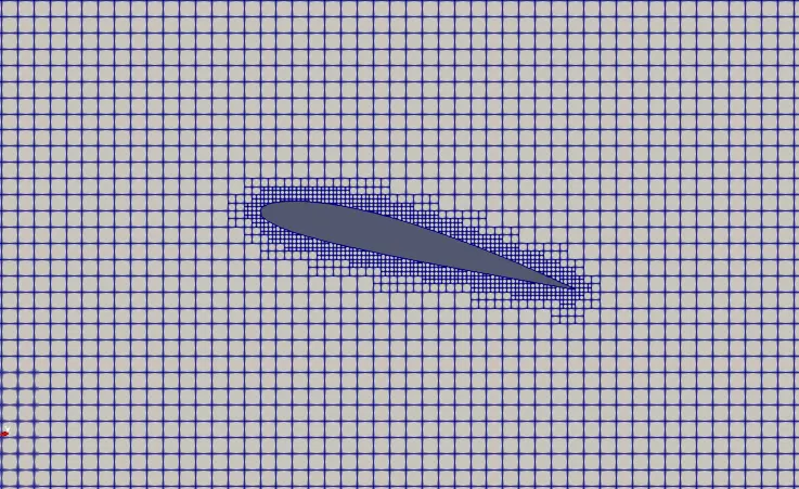
Snip of the base grid defined as well as the embedd layer applied is shown below,
* Time intervals for writing the 3D o/p file as well as the text file are defined under the output/processing. A snip of the same is shown below,
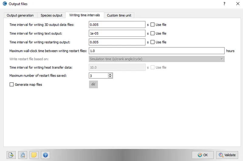
* This completes setting up of the case and then the simulation is run using the cygwin and the results are post-processed using paraview.
RESULTS:
Angle of attack = 1 degree :
* Geometry:
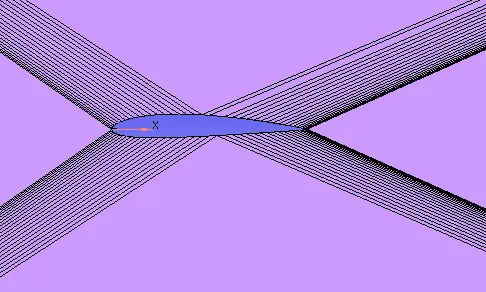
* Mesh generated:
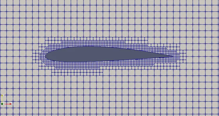
* Total cell count:
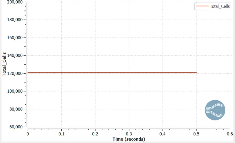
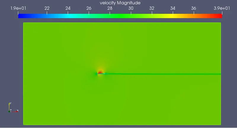
* Velocity contour:
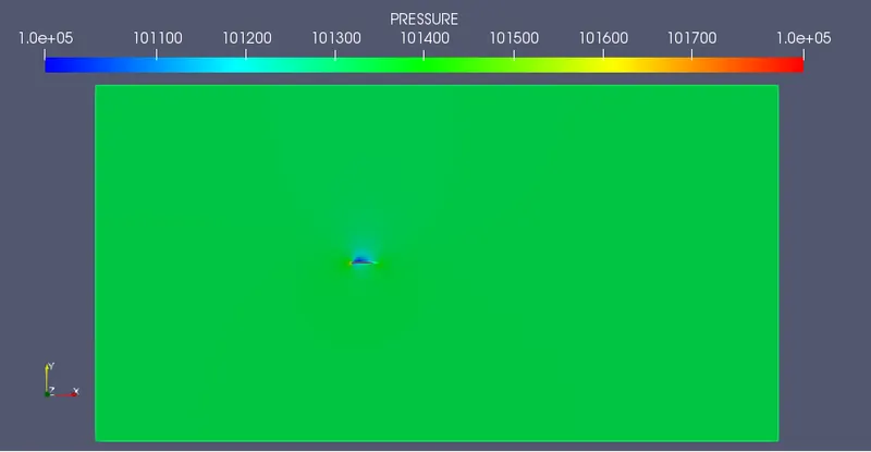
* Pressure contour:
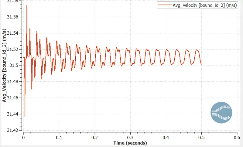
* Outlet velocity:
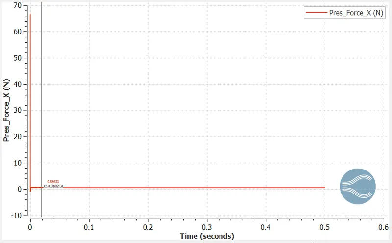
* P_x plot:
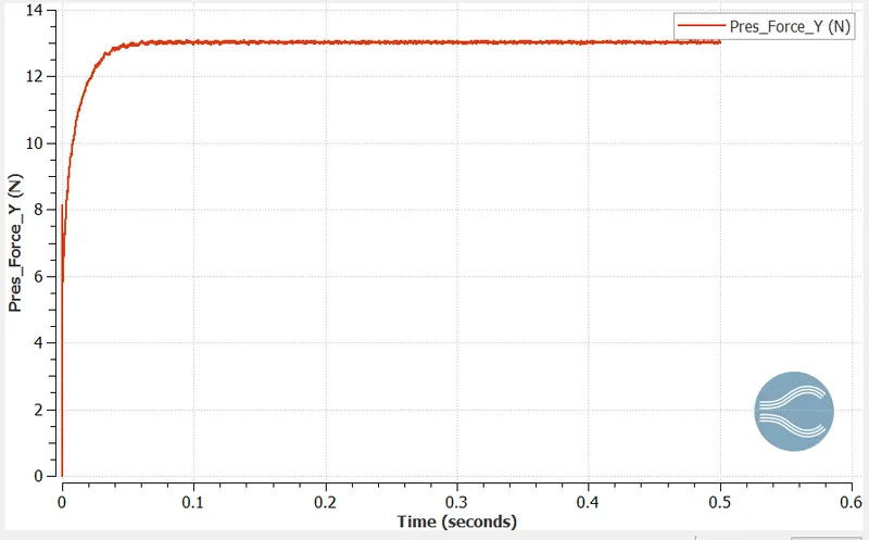
* P_y plot:
Angle of attack = 5 degree :
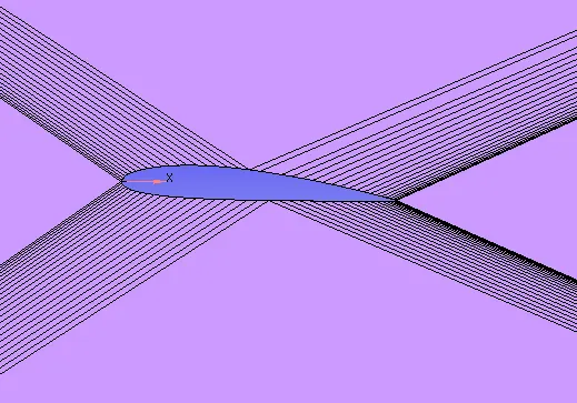
* Geometry:
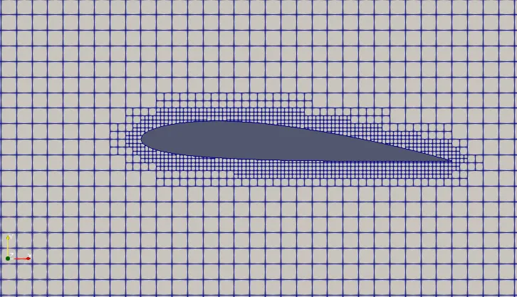
* Mesh generated:
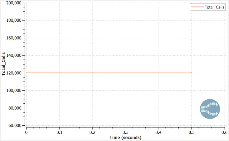
* Total cell count:
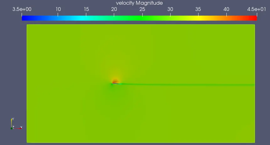
*Velocity contour:
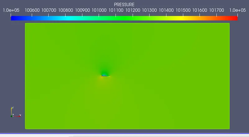
* Pressure contour:
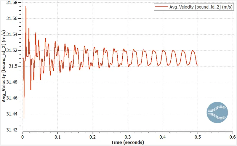
* Outlet velocity:
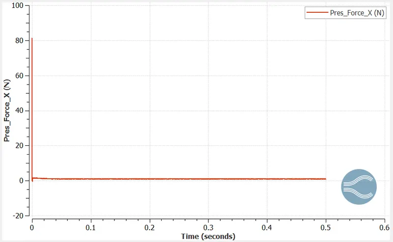
* P_x plot:
* P_y plot:
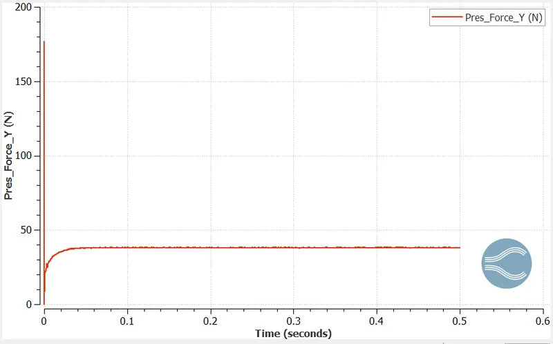
Angle of attack = 10 degree :
* Geometry:
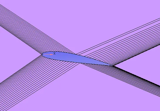
* Mesh generated:
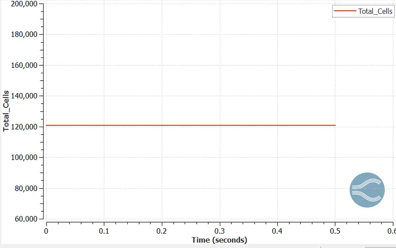
* Total cell count:
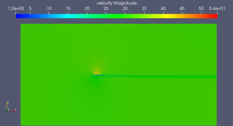
* Velocity contour:
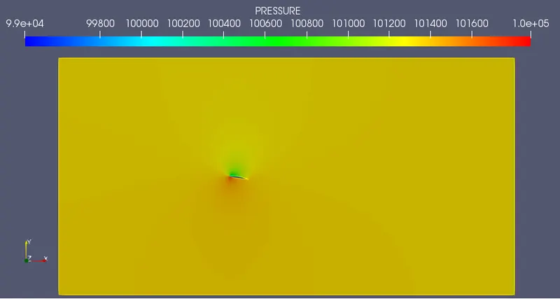
* Pressure contour:
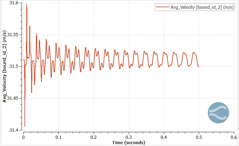
* Outlet velocity:
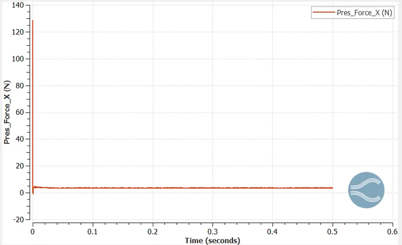
* P_x plot:
* P_y plot:
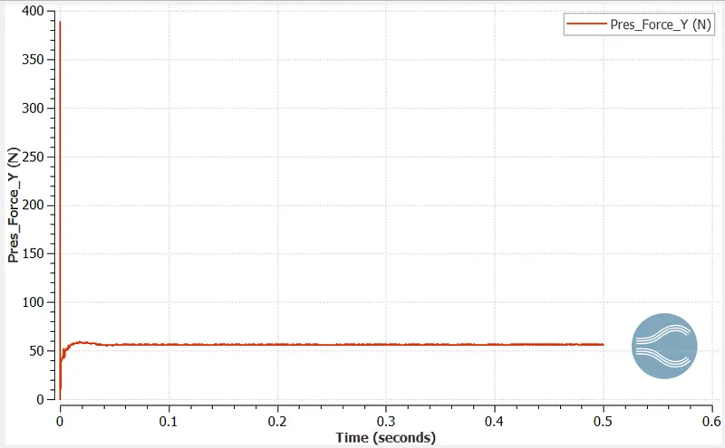
Angle of attack = 15 degree :
* Geometry:
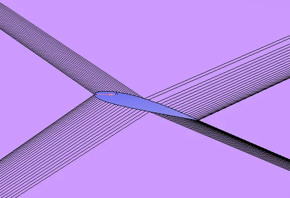
* Mesh generated:
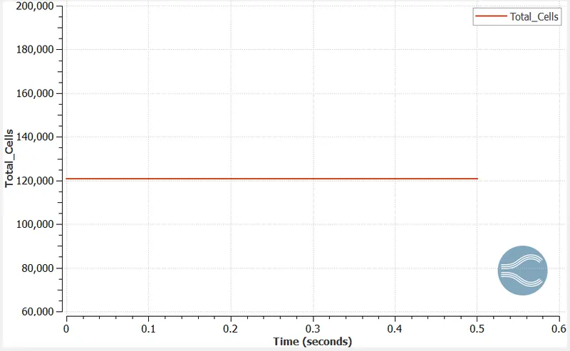
* Total cell count:
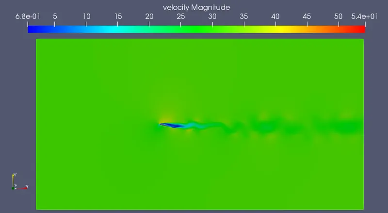
* Velocity contour:
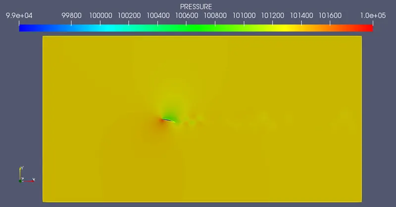
* Pressure contour:
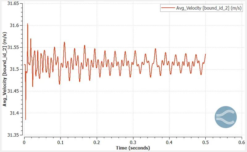
* Outlet velocity:
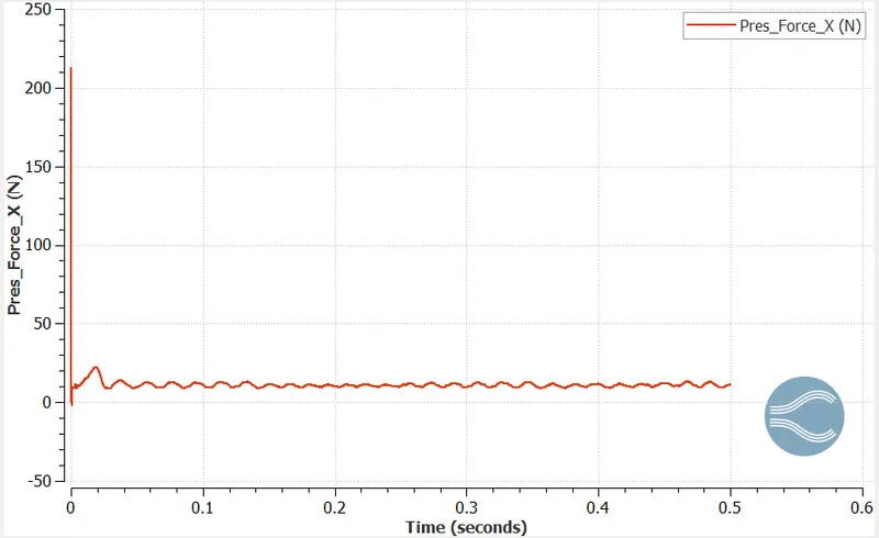
* P_x plot:
* P_y plot:
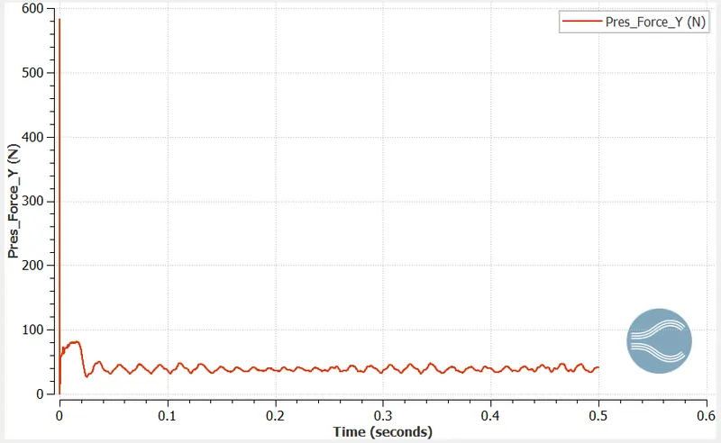
* From the above obtained data, Drag force, Lift force, coefficient of drag and lift are calculated using excel, a table showing the tabulated result is shwon below.

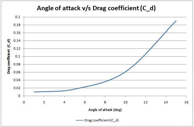
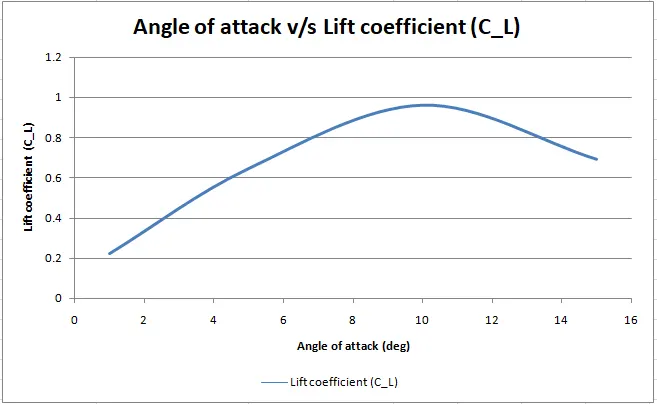
* It can be observed from the above plots that till the angle of attack is 10 degree the coefficient of lift as well as coefficient of drag increases, after that as the angle of attack increases the coefficient of lift decreases and coefficient of drag still increases, this condition is called stall.
* It is beacuse of flow separation and formation of wide wake region over the surface of the airfoil is the cause for stall.
* Stall is highly undesirable because there is increase of drag.