Gate Valve Parametric Study
#Aim:
* To paramaterise the valve opening from 10% to 80%.
* To calculate mass flow rates at different valve openings using parameters option in ansys workbench.
* To calculate the flow coefficient and flow factor for different mass flow rates of different valve openings.
#Introduction:
Control valves are common mechanical component that we come across in our daily life. Be it for the domestic household purpose or commercially profound industrial process control valves play an important role in regulating the flow of fluids. In simple words we can define control valves as mechanical components which are used to regulate/control the flow of fluids. Control of fluid flows can be achieved by varying the size of flow passage either manually or automatically. Manual controlling of control valve includes operating the hand wheel to open and close the flow passage. Automatic controlling involves operating using electric, hydraullic or pneumatic actuators.
Flow coefficient and flow factor are 2 parameters usually used to determine the efficiency of a valve. Flow coefficient of a valve is its relative measure of efficiency at allowing fluid flow through it.Flow coefficient is defined as volume of water at 60°F in gallons that will flow in 1 min across a valve with a pressure drop of 1Psi. It tells us how to properly size the valve so that it has minimum effect in hydraullic efficiency. Flow coefficient is usually denoted as Cv. Knowing the Cv value helps us in:
* Selecting a valve of proper size to match our application.
* Understanding the pressure drop across the valve.
Cv is calculated using the formula, `Cv = Q*sqrt((SG)/(DeltaP)`
where, `Q -` Flow rate (Gallons/min).
`SG -` Specific gravity of fluid`
`DeltaP -` Pressure drop across the valve (psi).
Flow factor is defined as flow rate in cubic meters per hour of water at a temperature of 16°C with a pressure drop across the valve of 1 bar. It is given using a formula,
`Kv = Q*sqrt((SG)/(DeltaP)`, it is metric equivalent of flow coefficient
where, `Q -`Flow rate (m^3/h).
`SG -` specific gravity.
`DeltaP -`Pressure drop across valve (bar).
`Kv -`m^3/h*bar^0.5
or Kv can also be calculated using the Cv and the formula is given as `Kv = 0.865 * Cv`[m^3*h^-1*bar^-0.5`
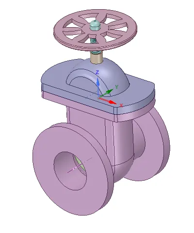
In this simulation water is used as the fluid which is passing through the valve. Valve used for the simulations is as shown below,
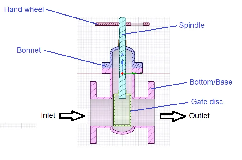
Different components associated with the above gate valve can be shown through a cut section,
#Simulations:
The control valve shown above is first opened in spaceclaim and the fluid volume is extracted. Below is the snip of the fluid volume.
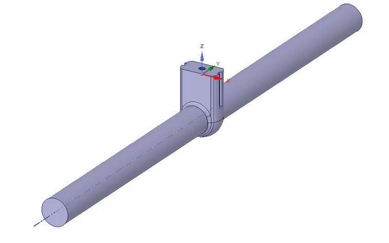
Above fluid volume is extracted in spaceclaim using volume extraction, then selecting 3 edges of bottom part of the valve. 3 edges which are used to extract the volume includes the inlet, outlet, the top opening of the base which matches with the bonnet. The fluid volume extracted can be further understood by observing the cut section as shown below.
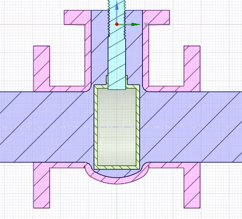
As the fluid moves from inlet to outlet, using the gate disc the flow of fluid is controlled. Movement of the gate disc is achieved using the spindle which inturn is connected to the hand wheel. By observing the above cross-section views we can understand that the gate disc is completley closing the passage, in other words we can say that there is no fluid passage at all. So the objective of the challenge is to give a lift of 10 mm to 80 mm to the gate disc and hence observe the mass flow rate, calculate the flow parameters flow coefficient and flow factor.
*Setup:
* First gate disc is moved 10 mm upwards, this creates a small flow passage for the fluid to flow through. Movement to the gate disc can be given using the move option in spaceclaim. Required distance can be typed and hence movement can be given to the gate disc. Below snipet shows the move option and the parametric option .
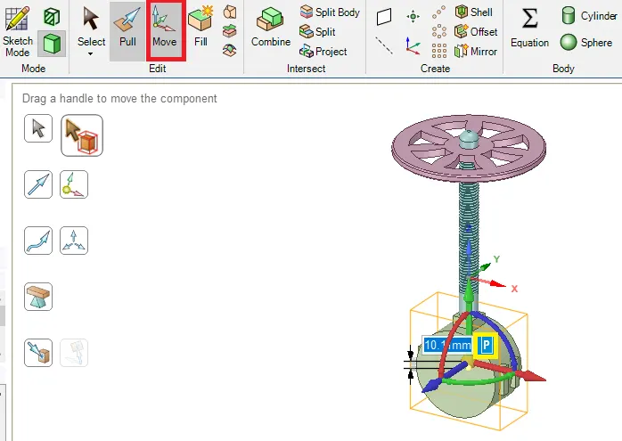
Move option as well as parametric options are highlighted in the above snipet. Using parametrise option, it is like for the given 10 mm lift what ever the meshing, boundary condition and all other post processing parameters are set to calculate mass flow rate same will be used when a movement of 20 mm to 80 mm is provided. The points from 20 mm to 80 mm are called design points.
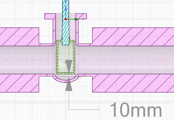
Below is the snip of the cross section after giving a 10 mm movement to the gate disc,
*Meshing:
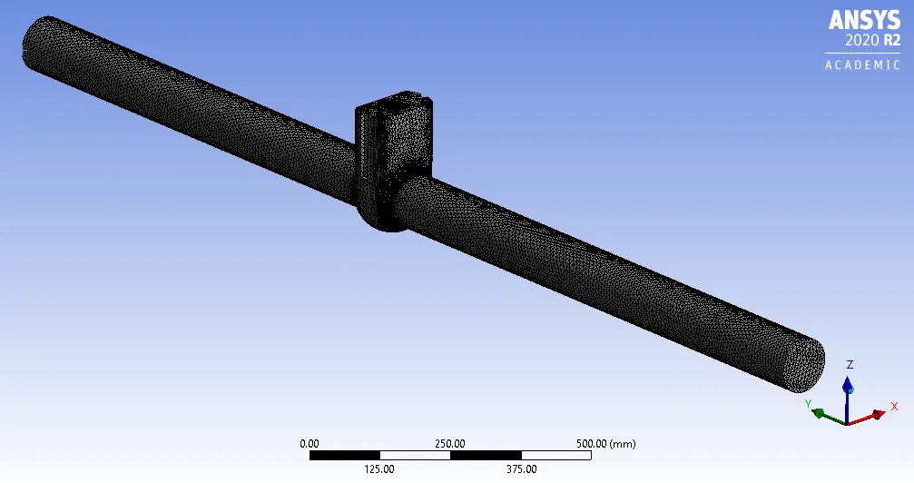
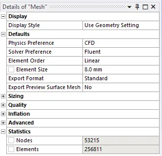
Fluid volume is meshed in the meshing module. Element size of 8 mm is provided and also an edge sizing is provided to the inlet and outlet edges by giving a total of 36 divisions. Mehsed fluid volume is as shown below:
below is the snipet of the mesh count:
* Solver setup:
Pressure based solver and steady state simulation is used. Gravity is applied in -z direction. Inlet boundary condition is set to pressure inlet and a value of 10 Pa is assigned. Outlet boundary condition was set as pressure-outlet and value of 0 Pa is set default by solver.
Before setting the flow model, it is important to calculate the Reynolds number and hence determine the flow model. Since pressure-inlet boundary condition is used for the fluid entering the inlet velocity is determined using 'options' which is under the solutions tab of the fluent. Since the fluid movement is in y-direction velocity at the inlet is obtained as 0.1415488 m/s.
Reynolds number, `Re = (U*D)/nu`
`U -` Inlet velocity (m/s).
`D -`Characteristic length, (Inlet diameter) (m).
`nu -`Kinematic viscosity of fluid (m^2/s).
Inlet diameter, D = 0.1 m, U = 0.1415488 m/s, since water is used as the fluid `nu`= 1.004 * 10^-6 m^2/s
therefore `Re = (0.1*0.1415488)/(1.004*10^-6) = 14.09*10^3`
for internal flow Re greater than 2300 is considered as turbulent flow, the flow under consideration is turbulent and hence K-ε turbulent model, realisable with scalable wall function is used.
The fluid volume is to be set as water in the cell zones. Apart from above setup, mass flow rate plot and velocity contour is set as output. Solution is run for 250 iterations and results are noted.
*Result:
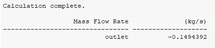
For gate lift of 10 mm the mass_flow_rate obtained, `dot m = -0.14944 (kg)/s`a grab of the same is provided below:
* Velocity contour:
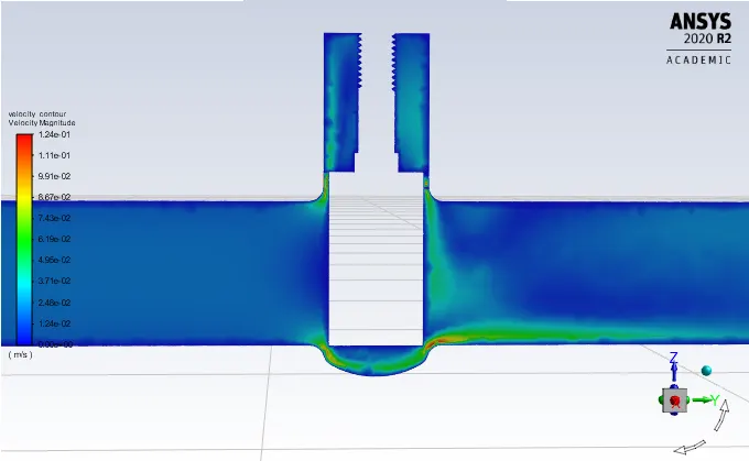
since our aim is to calculate the flow coefficient and flow factor it is calculated using the mass flow rate obtained,
Flow coefficient is given as, `Cv = Q*sqrt((SG)/(DeltaP)`
Since we have obtained mass flow rate, `dot m = -0.14944 (kg)/s` -ve sign can be ignored it implies that the fluid is flowing outside.
mass flow rate`dot m`needs to be converted into volume flow rate Q, Since the definition of Flow coefficient takes Q in gallons/min, Kg/s needs to be converted into Gallons/min
hence, Q = 0.14944/1000 m^3/s = 1.49*10^-4 m^3/s. This Q obtained in m^3/s is multiplied by 264.17 and 60 to convert m^3/s into gallons/min.
therefor Q = 2.34 gal/min.
SG = 1, since the fluid is water
`Delta P` = 0.00145 Psi, since the inlet pressure is 10 Pa and outlet pressure is 0 Pa the difference will be 10 Pa which is converted to Psi
therefore, `Cv = 2.34*sqrt(1/0.00145) = 62.2`
Flow factor, `Kv = 0.865 * Cv`
therefore, `Kv = 0.865*62.2 = 53.803` m^3*h^-1*bar^-0.5
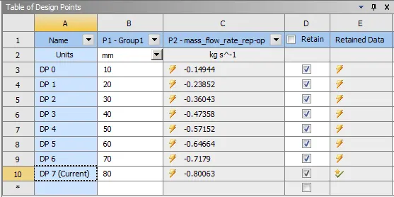
* Above steps completes the calculations concerned with 10 mm lift. For further lifts of gate disc from 20 mm to 80 mm parametric options is used. When parametrise option is clicked a parameter tab sets up under the Results tab. Using this parameters option we can enter different gate lifts as design points. Once all the design points are entered all the design points can be updated. Individually design points can be updated by right clicking and selecting 'Update selected design point' option. Once all the design points are updated we can right click on desired design point and can set it as current design point. Once any of the design point is set as current design point we can move to spaceclaim, mesh, fluent to view the geometry, meshing and the final results. All the contours, animations, plots, which are set for 10 mm lift will get updated as per the set current design point.
Below are the results obtained for different parametric design points:
1. For a lift of 20 mm:
Geometry:
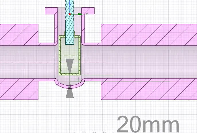
* Mass flow rate, `dot m = 0.2385 (kg)/s`

*Velocity contour:
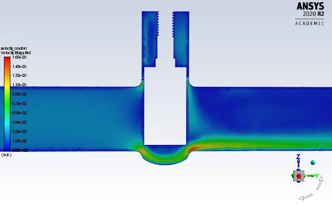
2. For 30 mm lift:
* Geometry:
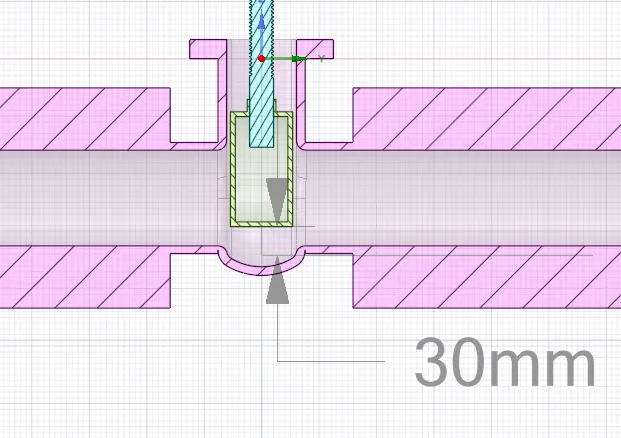
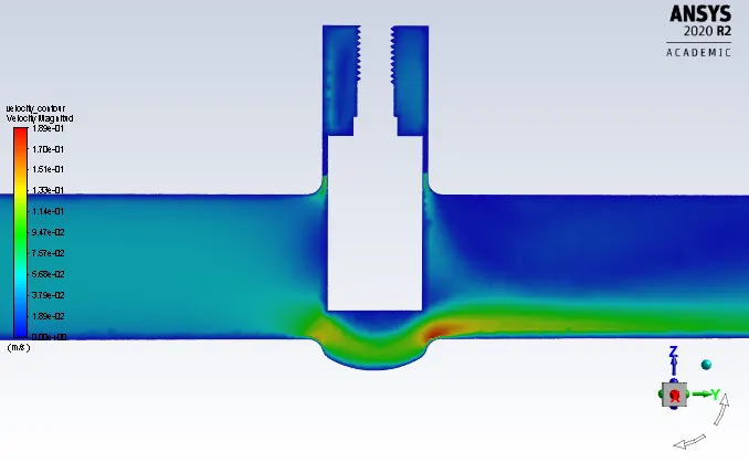
* Mass flow rate `dot m = -0.3604 (kg)/s`

* Velocity contour:
3. For 40 mm lift:
* Geometry:
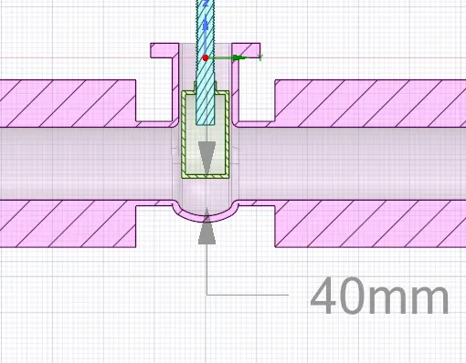
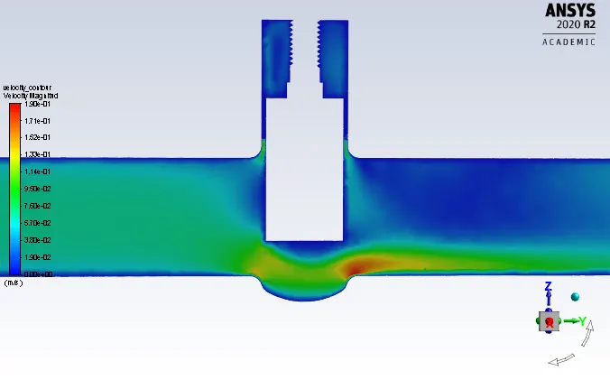
* Mass flow rate `dot m =-0.47357 (kg)/s`

* Velocity contour:
4. For 50 mm lift:
* Geometry:
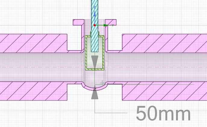
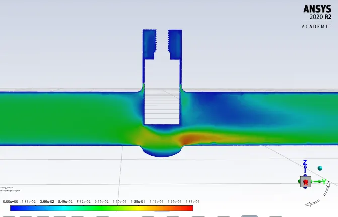
* Mass flow rate, `dot m = -0.571 (kg)/s`

* Velocity contour:
5. For 60 mm lift:
* Geometry:
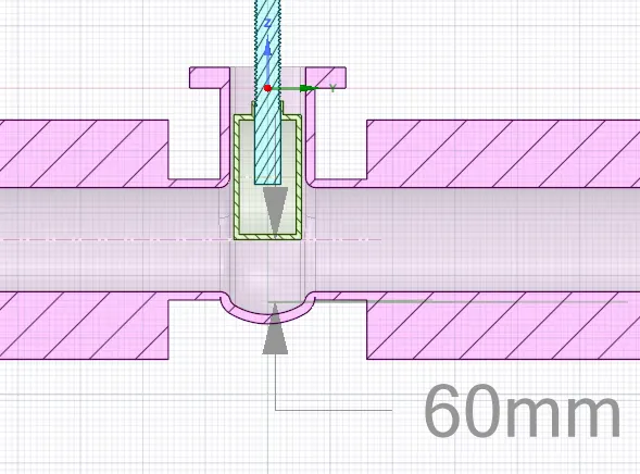
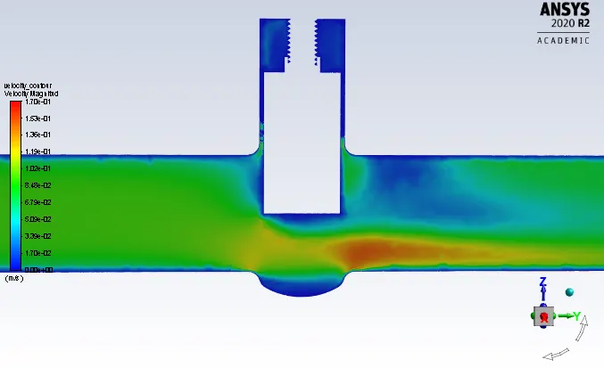
* Mass flow rate, `dot m = -0.646 (kg)/s`

*Velocity contour:
6. For 70 mm lift:
* Geometry:
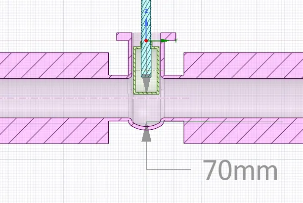
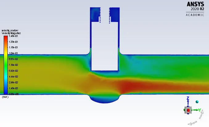
* Mass flow rate, `dot m = -0.717 (kg)/s`

* Velocity contour:
7. For 80 mm lift:
* Geometry:
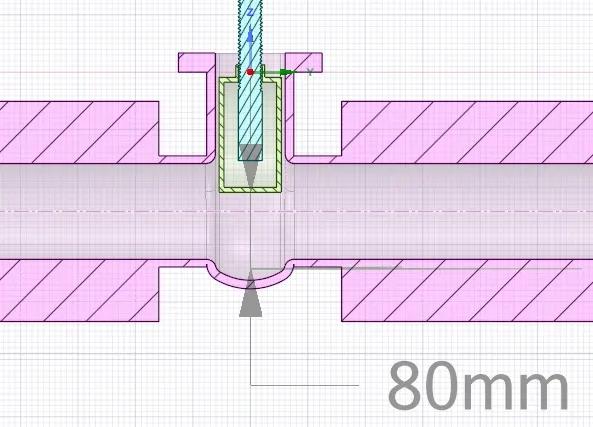
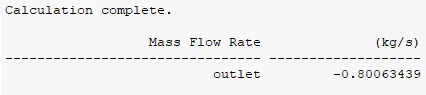
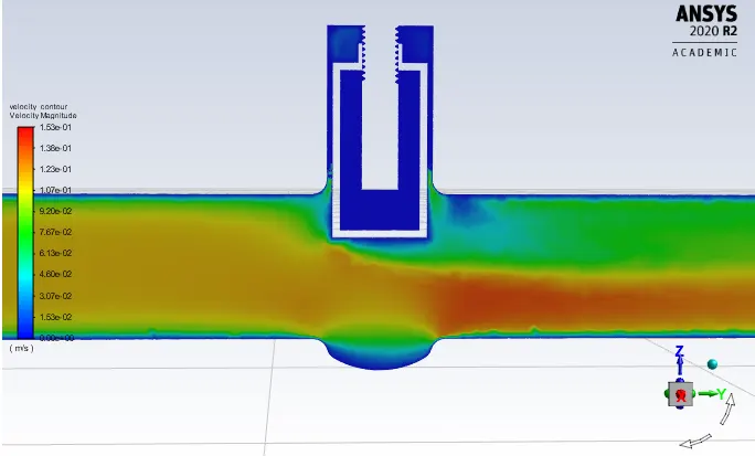
* Mass flow rate `dot m = -0.80063 (kg)/s`
* Velocity contour:
Above results for different valve openings are tabulated below along with flow coefficient and flow factor.
| Valve_opening | FLOW_RATE (kg/s) | `Cv` |
`Kv` [m^3/h*bar^0.5] |
| 10 mm | 0.1494 | 63.3 | 54.7 |
| 20 mm | 0.2385 | 101 | 87.36 |
| 30 mm | 0.3604 | 152.57 | 131.97 |
| 40 mm | 0.4735 | 200.6 | 173.57 |
| 50 mm | 0.5715 | 242.08 | 209.40 |
| 60 mm | 0.6466 | 273.58 | 236.90 |
| 70 mm | 0.7179 | 304.07 | 263.02 |
| 80 mm | 0.8006 | 339.07 | 293.30 |
*Below is the snip of the parametric window showing all the design points and corresponding mass flow rate
Below is plot of valve openings and the flow parameter, flow coefficient and flow factor:
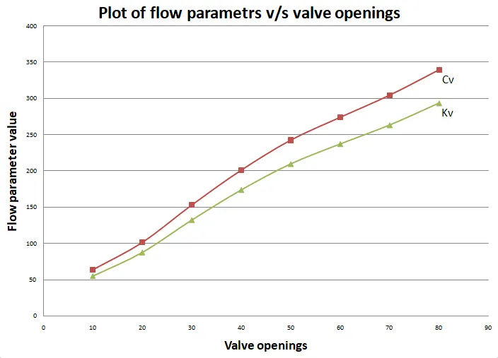
* From the above plot it is observed that as valve openings increases the value of Cv as well as Kv increases alomost linearly.