Week 3: Flow over a backward facing step
AIM
* To Simulate flow through a backward facing step for different mesh size.
* To identify recirculation region and hence obtain the velocity profile at that region.
* To obtain different plots such as pressure contour, velocity contour, mass flow rate etc.
INTRODUCTION
Flow separation taking place in an internal flow is of relevance as far as engineering applications are concerned. Flow separation in an internal flow takes place because of sudden change in the geometry which results in formation of recirculating region. Several experimental studies have been done in this regard to study the flow reversal in internal flow. Internal flow through a two dimensional backward facing step is the most accepted one because of its simple geometry.
2-D illustration of a backward facing step is shown below,

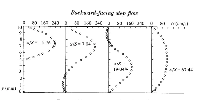
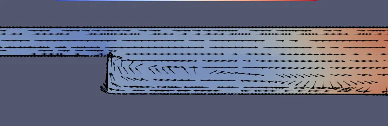
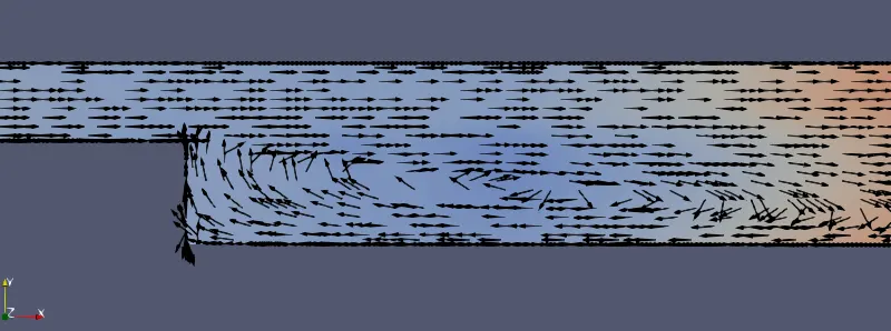
through the inlet the fluid flows into the volume, from the point where the step starts the geometry changes or in other words there is a sudden change in the cross-section because of this sudden change in the geometry the pressure increases and hence the flow reversal takes place. Flow reversal near the step region can be understood by observing the velocity profile or the velocity vector lines.
Velocity profile obtained from experimental studies is shown below, (Profile near the step region).
SIMULATIONS
* Geometry:
Geometry used in the geometry is an imported STL file. Geometry along with its dimensions (m) is shown below,
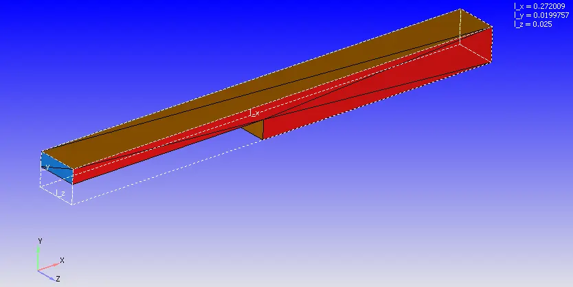
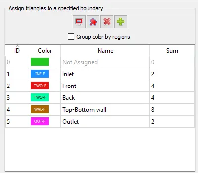
After creating or importing the geometry boundary's are flagged. In the above shown geometry the boundary's are flagged as Inlet, Outlet, Top-Bottom wall, Front and Back. A snip of the boundary flag along with the boundary id is shown below,
* Setup:
All the parameters required to run simulation is provided in the case setup. A snip of the case setup window is shown below,
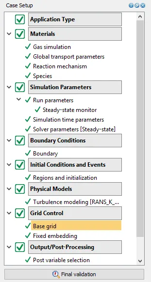
1. Application type: In this the we need to set wether the simulation is time based or crank angle based. Since this simuation does not involve any moving components it is set to time based.
2. Materials: Under this tab there are several parametrs. By clicking on the Materials tab we can set air as the fluid. Apart from this all the local controls which come under Gas simulation, Global tranport parameters, Reaction mechanism and Species is left as default.
3. Simulation parameters:
* Run parameters: Under this first comes the solver tab in which the solver type is set to steady state solver, simulation mode is set to full hydrodynamic and Gas flow solver is set as compressible. A snip of the same is provided below,
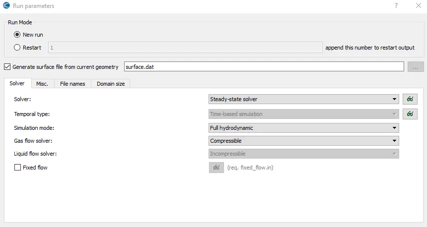
Second comes the Misc tab in which the steady state monitor is checked and Use shared memory is unchecked.
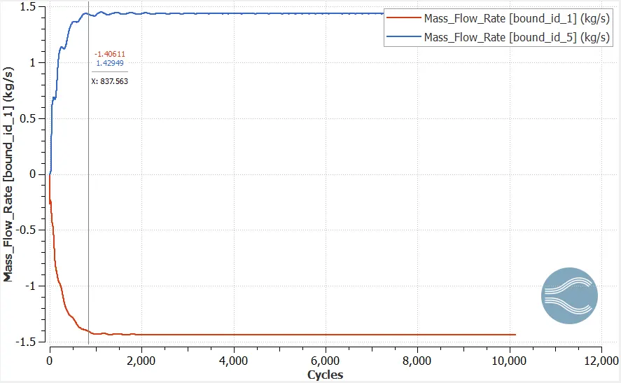
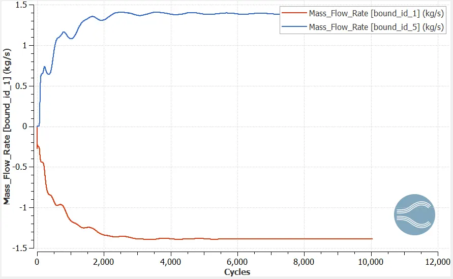
* Steady-state monitor: Under this mass fow rate at the outlet is set as the steady state monitor. Also the minimum number of cycles to be executed by the solveris set as 10000. Also the Monitor start delay and the Sample size is set as 200 and 100 respectivley, snip of the same is shown below,
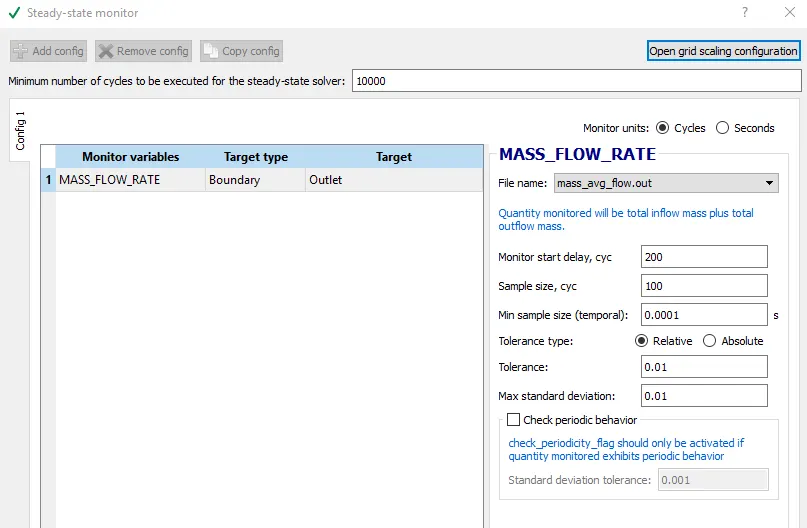
* Simulation time parameters: In here the start time for the simulation is set as zero. End time for simulation is set as 15000 cycles. Initial time step and minimum time step is set as 1e-6 cycles. Max time step is set as 2. Also the max convection CFL limit is set as 1. Apart from this all other local controls are left as default.
* Solver parameters: In this the steady state solver type is set as pressure based.
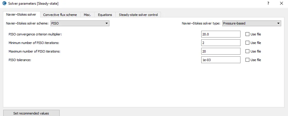
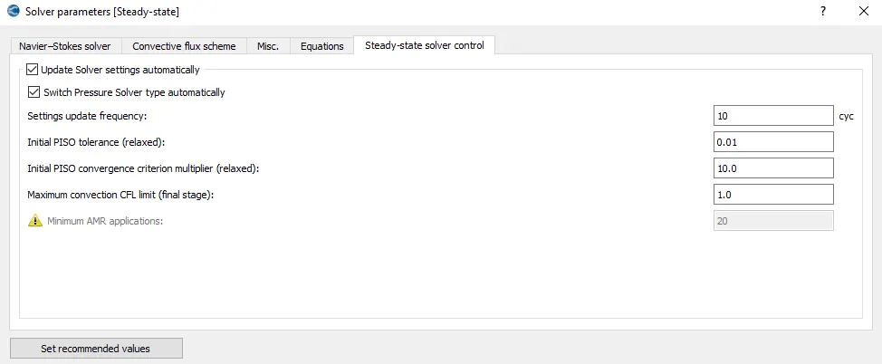
Also the Max convection CFL limit at final stage is set as 1.0.
4. Boundary Conditions (B.C):
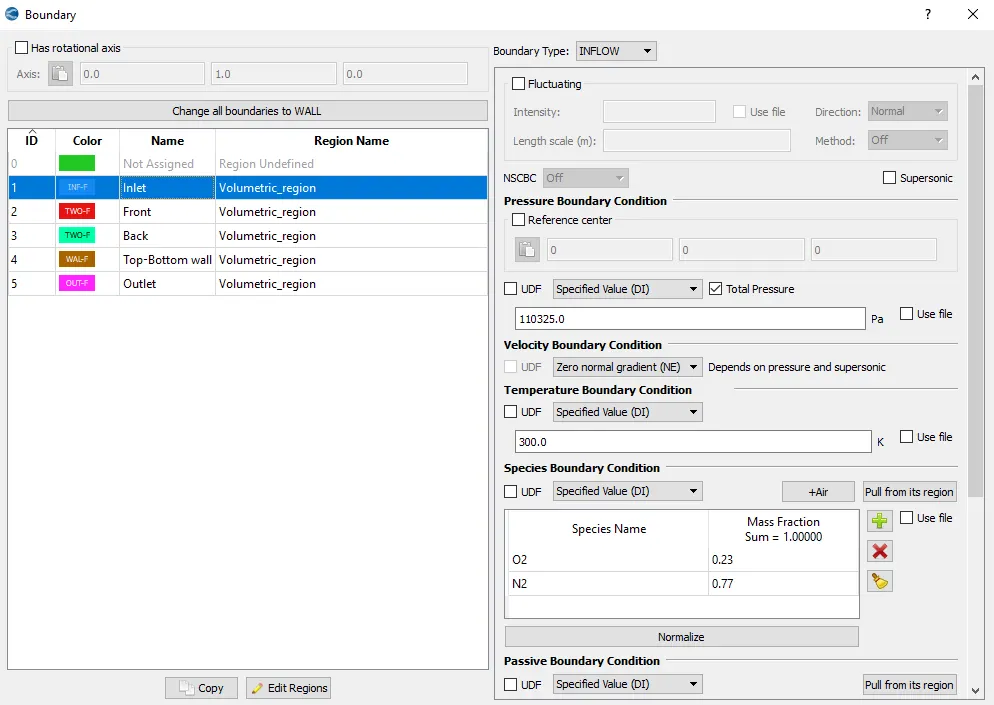
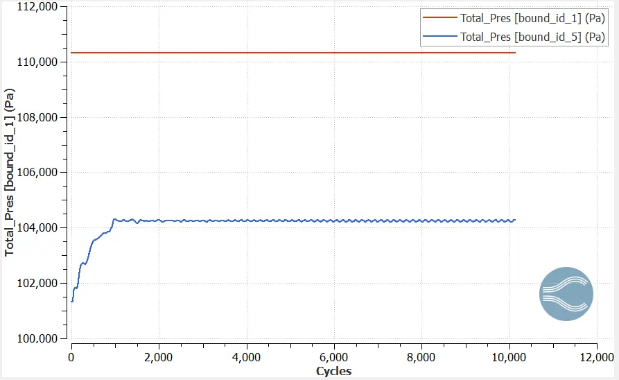
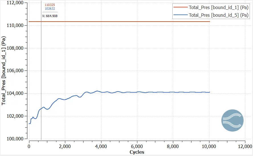
* Inlet: Pressure is set as 110325 Pa and inlet temperature is set at 300 K. Woking fluid air needs to specified along with mass fraction of the species.
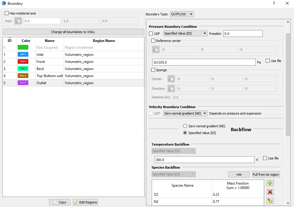
* Outlet: Pressure at the outlet is set as 101325 Pa. Temperature at the outlet is set as 300 K. Woking fluid air needs to specified along with mass fraction of the species.
* Front and Back: For both these faces 2-D is the B.C set.
* Top-Bottom wall: For this B.C is set as law of wall. Wall motion type is set as stationary also the surface movement is set as fixed. Temperature at the wall is set as 300 K.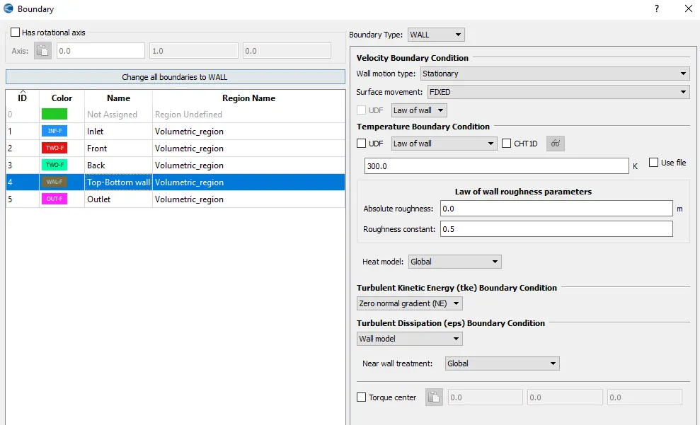
All the above mentioned Boundary's must belong to a volumetric region. Volumetric region is nothing but the entire fluid volume.
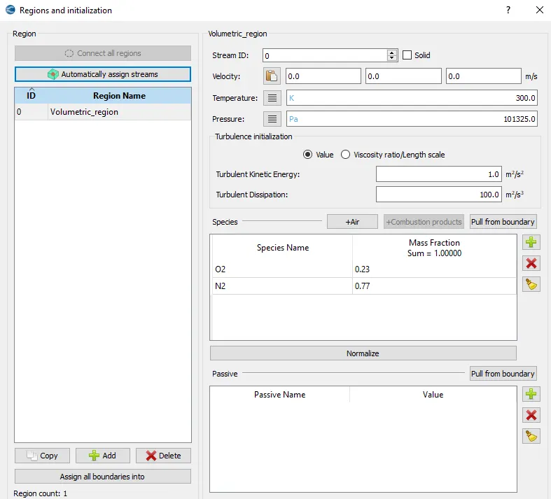
5. Regions and initialisation: Volumetric region is defined and initial conditions are set for all the cells present in the volumetric region. Volumetric region is initialised with pressure of 101325 Pa and a temperature of 300 K. Also the fluid under consideration needs to be specified here along with mass fraction of the species. A snip of the same is shown below,
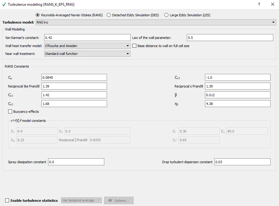
6. Physical models: In this the flow model can be set. For this simulation RNG K-ε turbulence model is used. All other local controls under this tab is left as default.
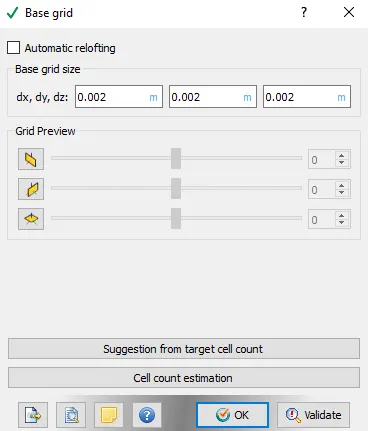
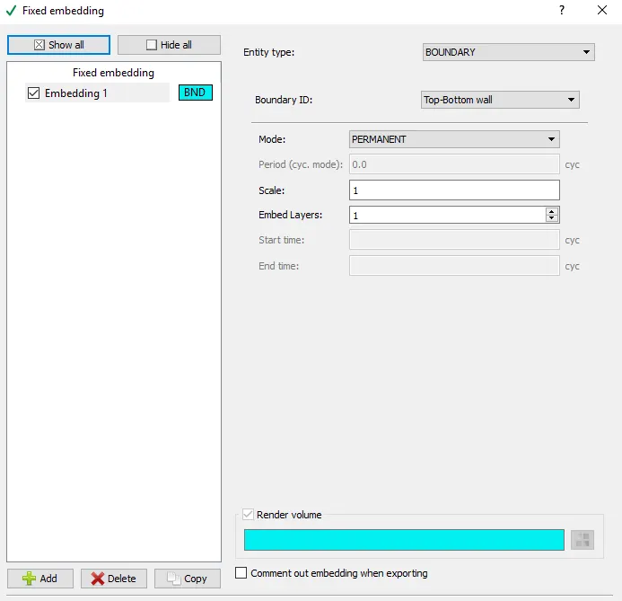
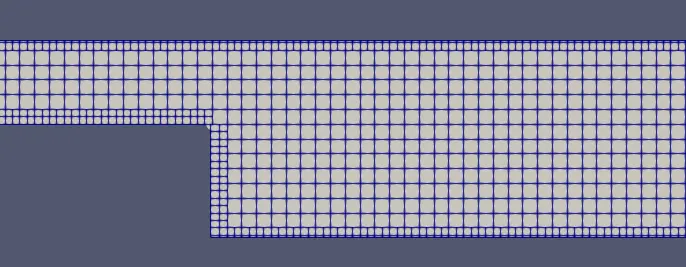
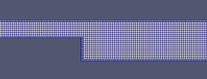
7. Grid controls: Grid sizing along x,y and z direction is specified here. For this simulation along with the grid sizing Fixed embedding is enabled. Fixed embedding can be enabled at any of the boundary's . In this simulation we are interested in capturing the the flow reversal fixed embedding is specified at boundary Top-bottom wall also a scale value of 1 is assigned, which means near the Top-bottom wall boundary the mesh size will be half of the mesh size mentioned in the grid sizing.
8. Output/Post-processing: Local controls under this tab is left as it is.
After setting up the simulation, "mpiexec.exe -n 4 converge-intelmpi.exe restricted" this command is executed in cygwin command window to run the simulation.
Simulation is run for 3 different mesh sizes, result obtained are disscussed below,
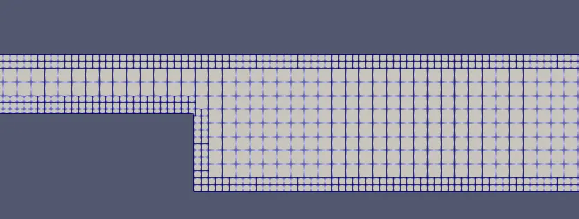
1. Mesh size = 2e-3.
* Mehsed surface:
* Velocity contour:
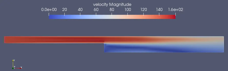
Velocity contour animation: https://youtu.be/3kwPJERaG9o
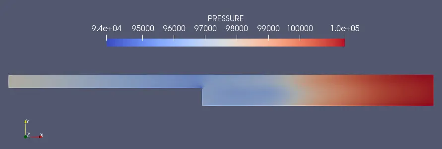
* Pressure contour:
* Velocity vector contour:
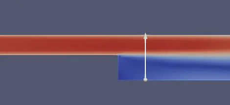
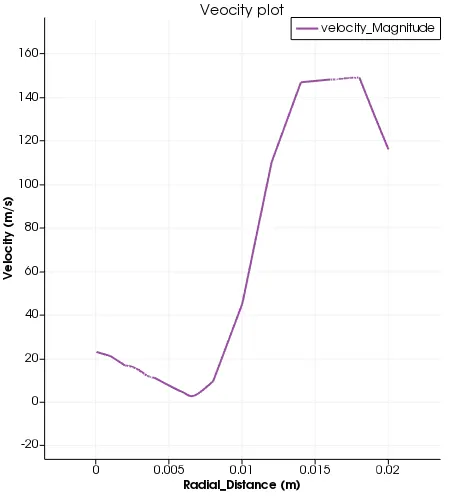
* Velocity profile at a distance of 0.136 m from inlet:
A snip of the line probe placed is shown below,
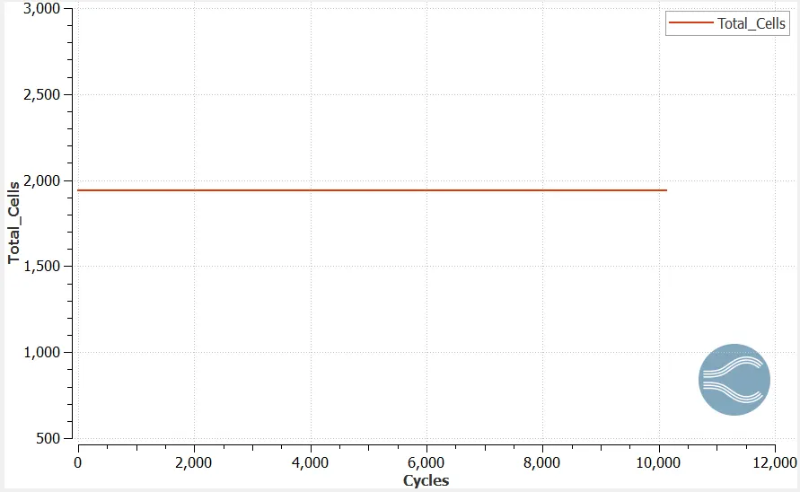
* Mesh count plot:
* Total pressure plot at inlet and outlet:
* Plot of mass flow rate at inlet and outlet:
2. Mesh size = 1.5e-3.
* Mehsed surface:
* Velocity contour:
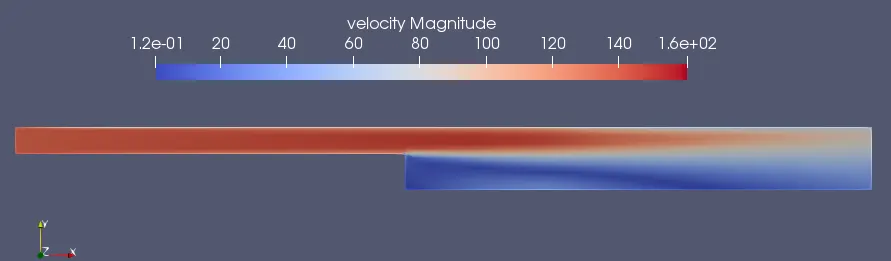
Velocity contour animation: https://youtu.be/AsYXcpNQA6A
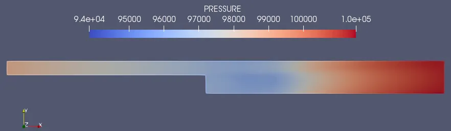
* Pressure contour:
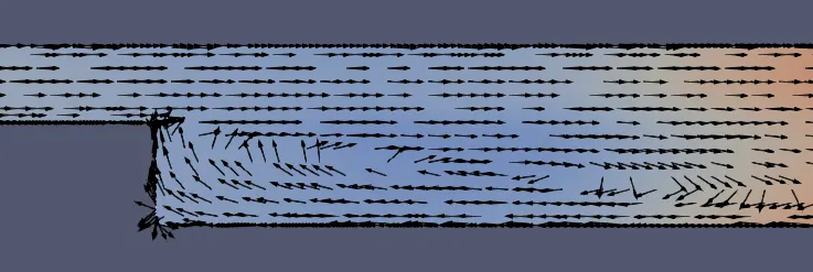
* Velocity vector contour:
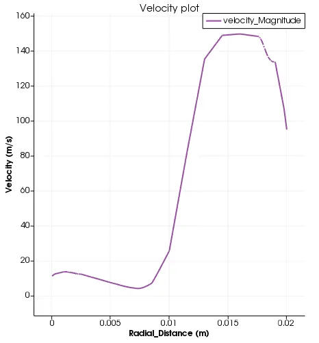
* Velocity profile at a distance of 0.136 m from inlet:
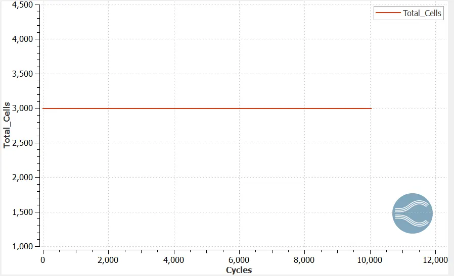
* Mesh count plot:
* Total pressure plot at inlet and outlet:
* Plot of mass flow rate at inlet and outlet:
3. Mesh size = 1e-3.
* Mehsed surface:
* Velocity contour:
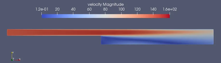
Velocity contour animation: https://youtu.be/HVdfgPKW27U
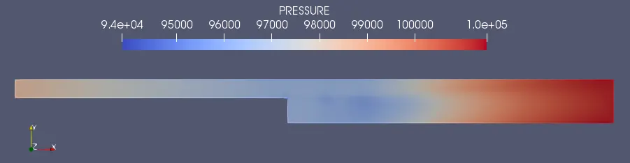
* Pressure contour:
* Velocity vector contour:
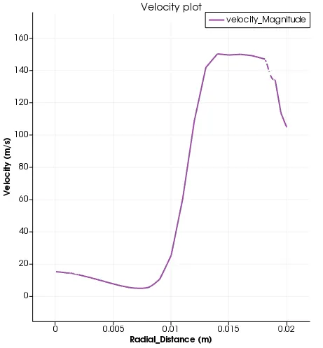
* Velocity profile at a distance of 0.136 m from inlet:
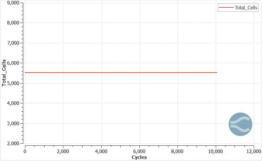
* Mesh count plot:
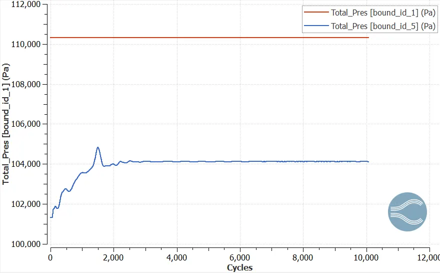
* Total pressure plot at inlet and outlet:
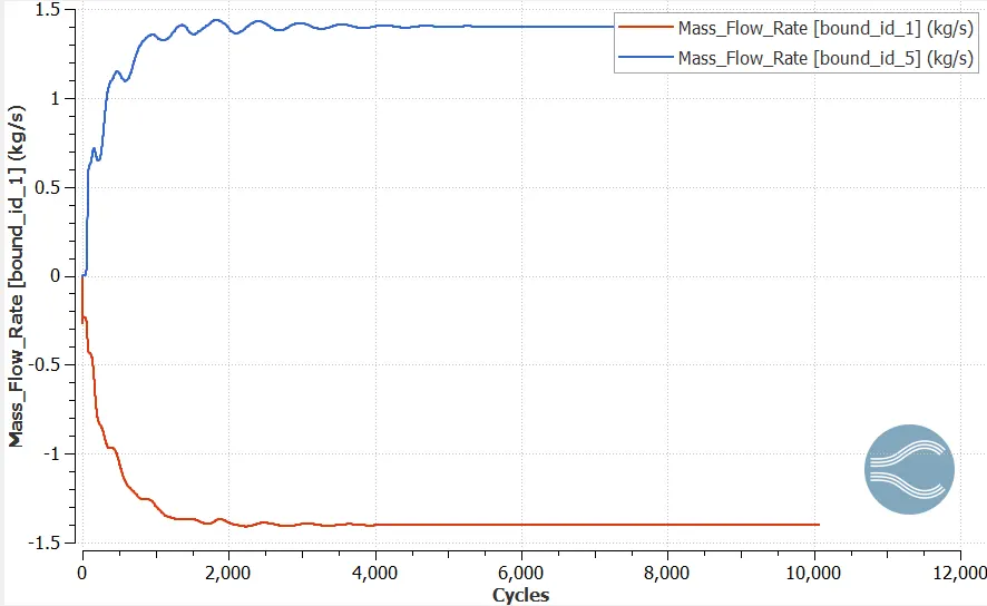
* Plot of mass flow rate at inlet and outlet:
CONCLUSION
* Velocity profile obtained matches with the velocity profile obtained from experimental studies, which implies that the result is correct.
* From pressure contour's it can be observed that as fluid flows from inlet to outlet there is a increase in total pressure, this increase in pressure takes place because of increase in cross section area of the geometry.
* Increase in total pressure is a resistance to the fluid flow or in other words we can say that the flow is through an adverse pressure gradient, which causes the flow reversal and hence recirculating region of fluid forms.
* Recircuating flow region can be clearly observed from velocity vector plot (glyph contour).