Week 6 - Multivariate Newton Rhapson Solver

AIM

* To solve given set of ode's using multivariate newton rhapson solver.

INTRODUCTION

It all starts with developing a good reaction mechanism. We know that combustion of fuel results in `CO_2, H_2O,N_2` and pollutants. The combustion reaction is not that straight forward, before the end products are formed there will be intermediary species formed and these intermediary species react with each other and hence elementary reactions takes place. A good reaction mechanism is the one which includes all the intermediary species and elementary reactions. Inorder to predict all the intermediary species and reactions accuratley we need to know the operating conditions such as pressure and temperature along with the reaction rate.

Determining reaction rate of a given reaction mechanism of real world combustion reaction is not a pen and paper work, for this computer needs to be used. Notations and matrices are used inorder to determine the reaction rates. End result of using notations and matrices gives us a matrix which has reaction rates of all the species.

Generally the matrix that we obtain is a matrix that has the reaction rates of the species, or in other terms those will be matrix of ode's. To solve this system of ode's we can apply euler's explicit method or euler's implicit method, as disscussed in the previous challenge applying explicit formulation is not that efficient since it is more dependent on the step size we take.

In this challenge a set of ode's are solved by applying implicit formulation on multivariate newton rhapson method. Newton rhapson method is used in root finding problems which has only 1 function, when more than 1 function is involved in root finding problem then multivariate newton rhapson method is used.

Multivariate newton rhapson method is given as, `X_n = X_o - alpha*J^-1*F`

where `J` is jacobian matrix and `F` is the column matrix of the root finding functions.

The system of ode's considered for this challenge as follows,

`dy_1/dt = -0.04*y_1 + 10^4*y_2*y_3`

`dy_2/dt = 0.04*y_1-10^4*y_2*y_3-3*10^7*y_2^2`

`dy_3/dt = 3*10^7*y_2^2`

Applying implicit formulation for the above ode system we have,

`(y_1^n - y_1^o)/(Deltat) = -0.04*y_1 ^n+ 10^4*y_2^n*y_3^n`

`y_1^n = y_1^o + Deltat*(-0.04*y_1^n + 10^4*y_2^n*y_3^n)`

`(y_2^n-y_2^o)/(Deltat) = 0.04*y_1^n-10^4*y_2^n*y_3^n-3*10^7*(y_2^n)^2`

`y_2^n = y_2^o + Deltat*(0.04*y_1^n-10^4*y_2^n*y_3^n-3*10^7*(y_2^n)^2)`

`(y_3^n -y_3^o)/(Deltat) = 3*10^7*(y_2^n)^2`

`y_3^n = y_3^o + Deltat*(3*10^7*(y_2^n)^2)`

so finally we have 3 equations in hand they are,

`y_1^n = y_1^o + Deltat*(-0.04*y_1^n + 10^4*y_2^n*y_3^n)`

`y_2^n = y_2^o + Deltat*(0.04*y_1^n-10^4*y_2^n*y_3^n-3*10^7*(y_2^n)^2)`

`y_3^n = y_3^o + Deltat*(3*10^7*(y_2^n)^2)`

these equations cannot be used as such in the newton rhapson method, these equations needs to be represented as root finding problems.

therfore, `f_1(y_1,y_2,y_3) = y_1^o + Deltat*(-0.04*y_1^n + 10^4*y_2^n*y_3^n) - y_1^n`

`f_2(y_1,y_2,y_3) = y_2^o + Deltat*(0.04*y_1^n-10^4*y_2^n*y_3^n-3*10^7*(y_2^n)^2) - y_2^n`

`f_3(y_1,y_2,y_3) = y_3^o + Deltat*(3*10^7*(y_2^n)^2) - y_3^n`

Above functions are used in multivariate newton rhapson technique to solve for `y_1, y_2,y_3`

Since the system of ode's considered is non-linear the jacobian matrix is used in the multivariate newton rhapson method

jacobian matrix, J = `[[(delf_1)/(dely_1), (delf_1)/(dely_2), (delf1)/(dely_3)],[(delf_2)/(dely_1),(delf_2)/(dely_2),(delf_2)/(dely_3)],[(delf_3)/(dely_1),(delf_3)/(dely_2),(delf_3)/(dely_3)]]`

Logic :

* First all three functions `f_1(y_1^o,y_1,y_2,y_3), f_2(y_1,y_2^o,y_2,y_3) and f_3(y_1,y_2,y_3^o,y_3)` are defined along with the jacobian matrix J`

* Since the jacobian matrix consists of partial derivatives of `f_1,f_2 and f_3`w.r.t `y_1,y_2,y_3`it is computed numerically rather than analytically`

* To compute the jacobian matrix analytically, taylor series expansion is used. To better explain how taylor series expansion is being considered is computing the jacobian matrix numerically let us consider the first term of the jacobian matrix, `(delf_1)/(dely_1)`

`f_1(y+Deltay) = f_1(y) + (delf_1)/(dely_1)*Deltay`

therefore `(delf_1)/(dely_1) = (f_1(y+Deltay)-f_1(y))/(Deltay)`

if we consider `f_1(y_1,y_2,y_3) = y_1^o + Deltat*(-0.04*y_1^n + 10^4*y_2^n*y_3^n) - y_1^n`, it has old as well as new value of `y_1`but the `Deltay` is only applied for the new `y_1`term.

* When taylor series expansion is applied we have the first term of the jacobian matrix given as

`(delf_1)/(dely_1) = y_1^o + Deltat*(-0.04*(y_1+Deltay_1)^n + 10^4*y_2^n*y_3^n) - (y_1+Deltay)^n` , same method is followed in computing other terms of the jacobian matrix`

if we consider the second term it would turn out as `(delf_1)/(dely_2) = y_1^o + Deltat*(-0.04*y_1^n + 10^4*(y_2+Deltay)^n*y_3^n) - y_1^n`

Similar way we can continue till the last term of the jacobian matrix.

* Two loops are defined one for time and other to check the tolerance criteria, since it is provided to run the simulation for 10 mins i.e, 600 seconds.

* A step size of 0.1 sec is selected, there are two reasons for the same. First reason is that for implicit formulation we can select any step size, irrespective of the step size selected the solution will be stable. Second reason for selecting a 0.1 sec time step is, starting from 1 sec to progress till 600 sec in intervals of 0.1 sec it will take 6000 time steps which will be a good time length for the solution to converge.

* F matrix is given as `F = [[f_1(y_1^o,y_1,y_2,y_3)], [f_2(y_1,y_2^o,y_2,y_3)] ,[f_3(y_1,y_2,y_3^o,y_3)]]`

* Since newton rhapson method has many matrix operations numpy module is imported, also since inverse of jacobian is used from numpy.linalg inv is imported.

Codes written to solve the above system of ode's is shown below:

"""
Solving a set of ODE using multivariate newton raphson method
"""
"""
	dy1/dt = -0.04*y1 + 10^4*y2*y3 - 3*10^7*y2^2
	dy2/dt = 0.04*y1 - 10^4*y2*y3 - 3*10^7*y2^2
	dy3/dt = 3*10^7*y2^2

"""
import numpy as np

from numpy.linalg import inv

def f1(y1_o,y1,y2,y3,dt):

	return (y1_o + dt*(-0.04*y1 + pow(10,4)*y2*y3) - y1)

def f2(y1,y2_o,y2,y3,dt):

	return (y2_o + dt*(0.04*y1 - pow(10,4)*y2*y3 - 3*pow(10,7)*pow(y2,2)) - y2)

def f3(y1,y2,y3_o,y3,dt):

	return (y3_o + dt*(3*pow(10,7)*pow(y2,2)) - y3)

def J(y1_o,y1,y2_o,y2,y3_o,y3,dt):

	dy = 1e-4

	J = np.ones((3,3))

	# Defining the first row of jacobian matrix
	J[0,0] = (f1(y1_o,y1+dy,y2,y3,dt) - f1(y1_o,y1,y2,y3,dt))/dy
	J[0,1] = (f1(y1_o,y1,y2+dy,y3,dt) - f1(y1_o,y1,y2,y3,dt))/dy
	J[0,2] = (f1(y1_o,y1,y2,y3+dy,dt) - f1(y1_o,y1,y2,y3,dt))/dy

	# Defining the second row of jacobian matrix
	J[1,0] = (f2(y1+dy,y2_o,y2,y3,dt) - f2(y1,y2_o,y2,y3,dt))/dy
	J[1,1] = (f2(y1,y2_o,y2+dy,y3,dt) - f2(y1,y2_o,y2,y3,dt))/dy
	J[1,2] = (f2(y1,y2_o,y2,y3+dy,dt) - f2(y1,y2_o,y2,y3,dt))/dy

	# Defining the third row of jacobian matrix
	J[2,0] = (f3(y1+dy,y2,y3_o,y3,dt) - f3(y1,y2,y3_o,y3,dt))/dy
	J[2,1] = (f3(y1,y2+dy,y3_o,y3,dt) - f3(y1,y2,y3_o,y3,dt))/dy
	J[2,2] = (f3(y1,y2,y3_o,y3+dy,dt) - f3(y1,y2,y3_o,y3,dt))/dy

	return J

"""
Defining initial conditions
"""
y1 = 1
y2 = 0
y3 = 0

"""
Defining the Y matrix
"""
y_old = np.ones((3,1))

y_old[0,0] = y1
y_old[1,0] = y2
y_old[2,0] = y3

"""
Defining the F matrix
"""
F = np.copy(y_old)

y_new = np.copy(y_old)


"""
Defining the tolerance
"""
tol = 1e-4

"""
Defining the relaxation factor
"""
alpha = 1

t_total = 600

dt = 0.1

L_1 = []
L_2 = []
L_3 = []
iter =1
repitation= []

a = np.arange(1,t_total,dt)

for i in range(0,len(a)):
	
	"""
	Defining the error
	"""
	error = 9e9

	while(error > tol):

		F[0,0] = f1(y_old[0,0],y_new[0,0],y_new[1,0],y_new[2,0],dt)
		F[1,0] = f2(y_new[0,0],y_old[1,0],y_new[1,0],y_new[2,0],dt)
		F[2,0] = f3(y_new[0,0],y_new[1,0],y_old[2,0],y_new[2,0],dt)

		y_new = y_old - alpha*np.matmul(inv(J(y_old[0,0],y_new[0,0],y_old[1,0],y_new[1,0],y_old[2,0],y_new[2,0],dt)), F)

		error = max(abs(y_new-y_old))
		print(error)
			
		y_old = y_new
	
		log_message = 'repitation No. = {0} y1 = {1} y2 = {2} y3 = {3}'.format(iter,y_new[0],y_new[1],y_new[2])
		print(log_message)
		
		L_1.append(y_new[0])
		L_2.append(y_new[1])
		L_3.append(y_new[2])

		iter = iter+1
		repitation.append(iter)
		

When above code is run we get the following output,

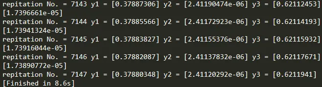
Observation :

* From the result obtained it is clear that for last few iterations the value of `y_1, y_2, y_3` are constant and hence the solution has converged.