Week 5 - Rayleigh Taylor Instability

Aim:

To simulate Rayleigh Taylor Instability using Ansys Fluent

Objectives:

1. Brief introduction to Rayleigh-Taylor Instability and CFD models based on Rayleigh-Taylor waves.
2. Defining Atwood number and calculating it for air-water and custom-fluid-water systems.
3. Create geometry and generate conformal meshes for analysing the grid dependence of the R-T instability for air-water system.
4. Run a simulation with water adnd custom fluid for the R-T instability with the refined mesh.
5. Analyse the animation of the R-T unstable flows with Atwood number theoritical predicitions.

Introduction:

Rayleigh-Taylor instability is observed in multiphase systems where a non-equilibrium initial condition such as heavier fluid is on top of lighter fluid. The instability grows with time in presence of the gravitational field to reduce the system's potential energy. The evolution of the instability can be characterised in two modes: the linear and the non-linear growth phase. In the linear phase, from linear pertubation analysis, we can predict the formation of small wave-like structure which grows in amplitude with time. This eventually gives rise to plume of the low-density fluid to rise in the heavier fluid and spikes of heavy fluid in the bulk of the lighter fluid. Eventually, the growth of the amplitude of the wave-like disturbances grow so large that non-linear terms in linear pertubation analysis cannot be further disregarded. These instabilites are observed ubiquitously in nature. Few of them are: mushroom clouds from volcanic eruptions, supernovas, instabilities in plasma fusion reactors.

Several CFD models are based on the linear analysis of the Rayleigh-Taylor waves. They are discussed very briefly as follows:

• Mass diffusion model
  • Describes the transport of mass and energy due to model viscosity and hence drives actual mixing in the fluids.
  • Works also for R-T unstable configuration, as mixing can be dominated by diffusion f the viscosity is sufficiently large.
• Variations of Single Fluid model
  • Potential flow model
    • Valid till early non-linear stage but limited to Atwod number of 1.
    • Single mode pertubations expands the flow equations to second-order around the bubble tips, obtaining an ODE for the bubble velocity.
  • Buoyancy drag model
    • Valid at all Atwood number but limited to non-liner stages of the instability.
    • ODE to evolve the width of the mixing layers
    • Bubble or spike amplitudes are described by balancing the inertia, buoyancy and drag forces.
    • Cannot model multiple mixing interfaces, cannot be easily extended to 2 or 3 dimensions and as a rule do not address demixing, also known as counter gradient transport.
  • Besnard-Harlow-Rauenzahn (BHR)
    • Advanced version of the single fluid model.
    • Based on evolution equations arising from second-order correlations and gradient-diffusion approximations.
    • Using a mass-weighted averaged decompostion, the original BHR model includes full transport equations for the Reynolds stresses, turbulent max-flux velocity, density fluctuations and turbulent kinetic energy dissipation rate.
• Variations of Multi-Fluid model
  • Use a separate set of equations for each fluid in addition to the main flow equations and provide an accurate modeling framework for demixing by correctly capturing the relative motion of the different fluid fragments.
  • Two equation k-l turbulence model
    • Provide equations for turbulent kinetic energy k and turbulent length scale l.
    • Derivied from buoyancy-drag models for self-similar growth of RT instabilities.
  • Three equation k-l-a turbulence model
    • Additional equation for turbulent mass-flux velocity considered.
  • Four equation k-l-a-b model
    • An extension of three equation model by including a fourth equation for density specific volume covariance.
    • Accurately reflect the effects of the changes in the density fluctuations.

Atwood number is defined as the ratio of the difference of the densities and the sum of the densities in density stratified flows. Mathematically, it is represented as follows

`A={rho_1 - rho_2}/(rho_1 + rho_2)`

where, `rho_1` depicts the heavier fluid and `rho_2` is the density of the lighter fluid.

For the air-water system,

`rho_1=998.2\ {kg}/m^{3}`

`rho_2=1.225\ {kg}/m^{3}`

`A=0.998`

For the custom-fluid-water system,

`rho_1=998.2\ {kg}/m^{3}`

`rho_2=400\ {kg}/m^{3}`

`A=0.428`

The behavior of the Raylor-Taylor instability is highly dependent on the Atwood number. As mentioned earlier, there are two stages of evolution, the linear regime, transition to non-linear regime via formation of the mushroom head or bubble formation and the non-linear regime characterized by the bubble merging and mixing. For lower Atwood number, the linear disturbances duration are longer and the mushroom head shape remain symmetrical. On the other hand, the for large atwood number the transition to the non-linear regiome is more aggressive.

In this study, we will try to validate these experimental observations using simulations in Ansys Fluent.

Geometry:

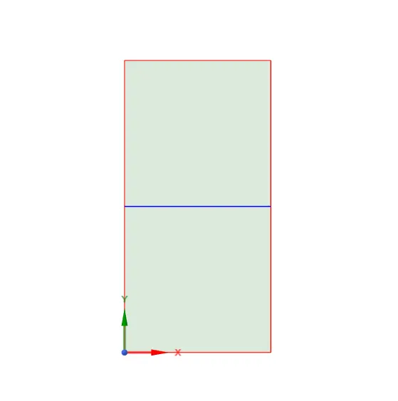
The geometry for all the three simulations is identical. It consists of two dimensional box with upper half of the rectangle is marked for heavier fluid which is water in this study and the lower half consists of the air or the custom fluid which plays the role of the lighter fluid. To generate a conformal mesh, we share the topology of the compuational domain. The height of the domain is 40 mm while the width is 20 mm. The computational domain is visualized as follows:

Meshing:

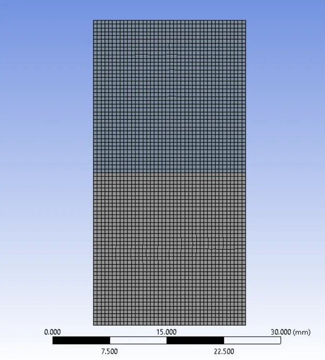
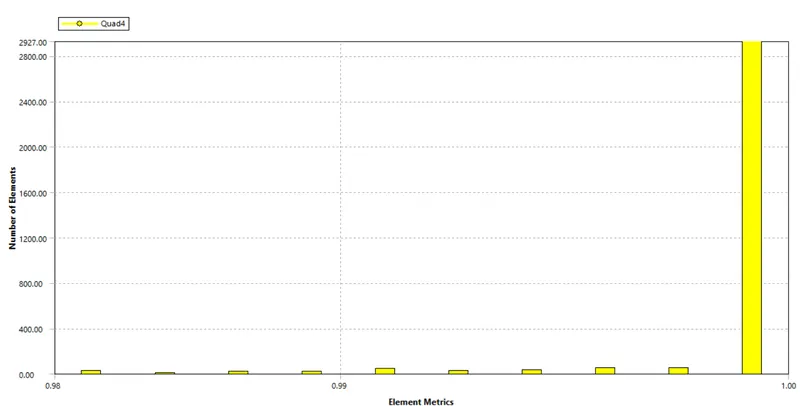
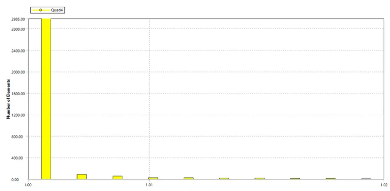
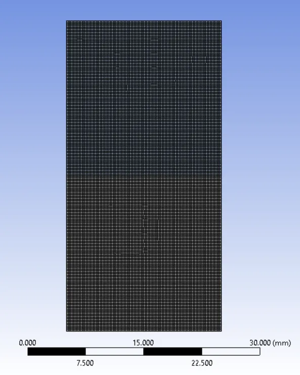
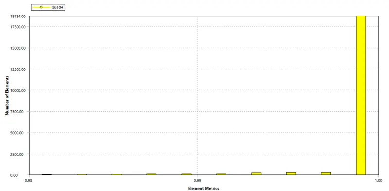
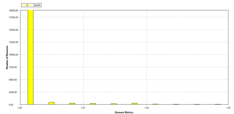
Because of the simple structure of the domain, the mesh is hex-dominant. This is good as it improves the mesh quality and reduces the mesh skewness. In this study, we consider two meshes: Base mesh and Refined mesh. The element size in the base mesh if 0.5 mm while the element size in the refined mesh is 0.2 mm. The details and the analysis of both the meshes is as follows:

Mesh 1:

• Mesh figure

• Element quality

• Aspect ratio

Mesh 2:

• Mesh figure

• Element quality

• Aspect Ratio

Casesetup:

The case setup for all the three cases is identical. We will depict the case settings from the ANSYS Fluent GUI in this section.

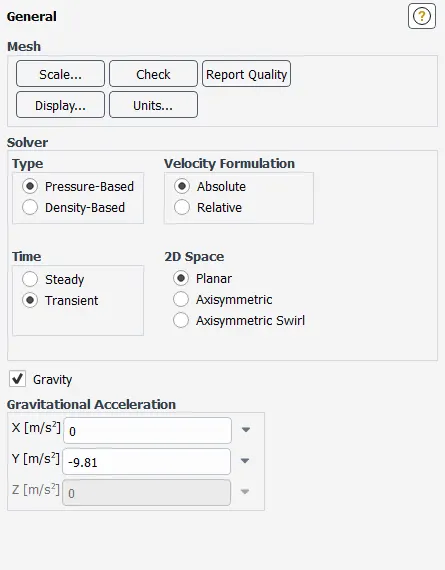
• General
  • We use a pressure-based transient solver as the growth of the instability on the interface is dependent on time.
  • We also consider gravitational force acting in the negative Y direction.

• Models
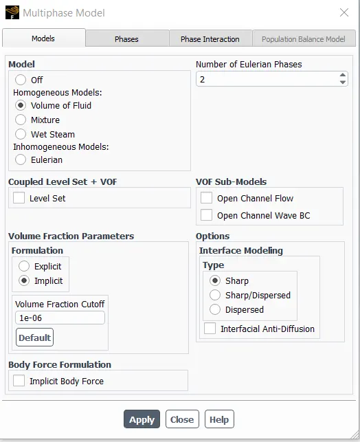
  • We consider implicit formulation of volume of fluid method to model the interface of the density stratified flows.
  • The phase 2 is water while the phase 1 is the air/custom-fluid.

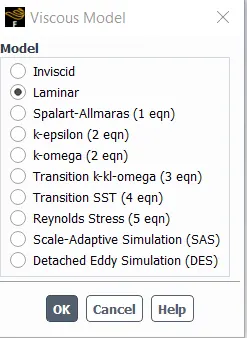
• We use laminar viscous model as the velocity scales are low enough such that no modeling of turbulence is required.

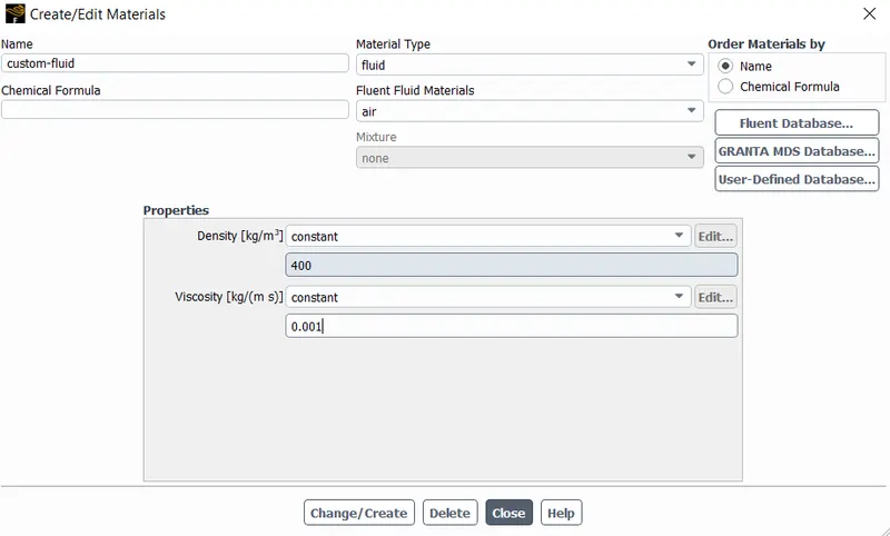
• Materials
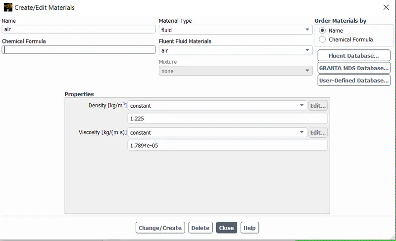
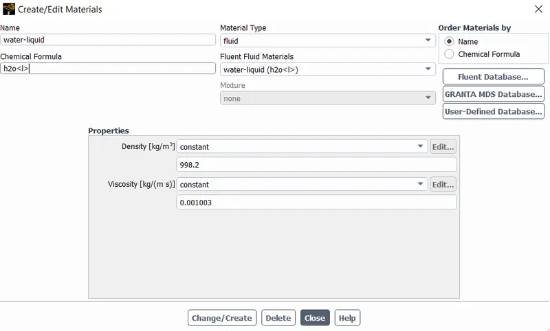
  • For the heavier fluid we use water from the Fluent database and for the lighter fluid we use the custom-fluid or air.

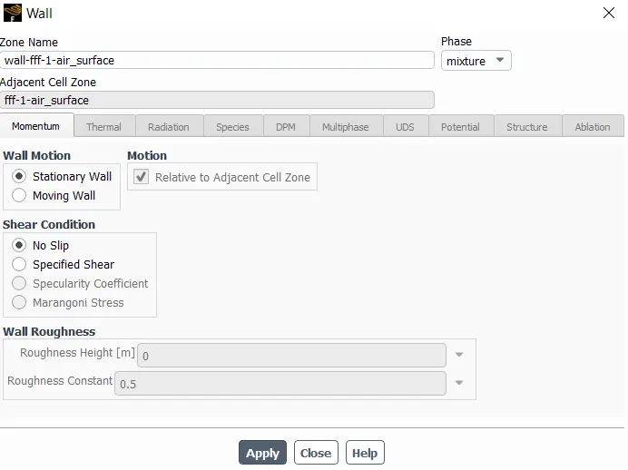
• Boundary Conditions
  • All the walls are stationary with no-slip condition

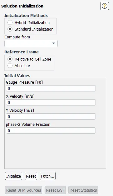
• Initialization
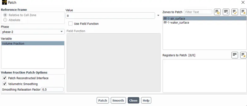
  • A standard initialization is provided.
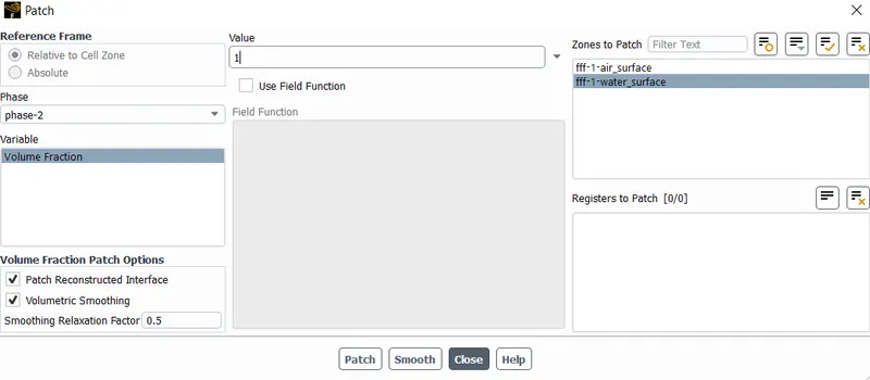
  • A patch of value 1 of heavier fluid in the upper half of the domain and the patch of value 0 of the heavier fluid in the lower half of the domain is provided to make the flow density stratified.

• Calculations
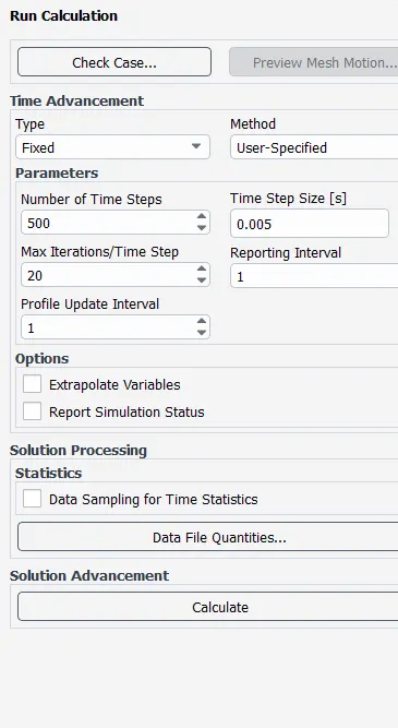
  • We run the simulations for 500 timesteps and each timestep of 0.005 seconds.

Simulation results:

Animation link of the baseline mesh: Baseline Animation Link

Animation link of the refined mesh: Refined Animation Link

Animation link of the custom-fluid water configuration: Custom Animation Link

Conclusions:

From the animations we can derive the following conclusions

1. Simulations for the refined and the base mesh reach to equilibrium conditions, hence bothe meshes provide reasonable results
2. The interface is diffused by a higher proportion in the bash mesh because of the numerical diffusion associated with larger cell sizes.
3. The simulation of air-water system shows that configuration quickly evolves into the non-linera regime which is expected.
4. The simulation of the custom-fluid-water configuration shows that the simulation is symmetrical and linear for longer amount of time than the air-water system. This is in trend because of the low Atwood number.