Week 4.1: Project - Steady state simulation of flow over a throttle body

Aim:

To setup and run steady state simulation for flow of air in a elbow pipe containing a throttle body.

Objectives:

• Generate mesh with suitable number of cells, appropriate scaling and embedded layers to accurately capture flow physics around the throttle in CONVERGE Studio
• Setup a steady state case for simulating the flow through the elbow pipe with the throttle at completely open position in CONVERGE Studio.
• Postprocess the converged results by plotting line plots and contours in Paraview and CONVERGE Studio.

Theory:

The throttle valve operates by obstructing ("throttling') the fluid flow in a channel to control the flow rate. It is one the most common and easily implementable flow control devices used in industries where handling the fluid flow is of crucial importance. The device working principle is based on the position of the valve which can vary from providing virtually zero obstruction to completely chocking a pipe.

In the current study, we simulate flow through an elbow pipe containing a butterfly throttle valve. The mechanism which obstructes the flow in butterfly valve is a circular disk. Although the model is quite simplistic in design, it proves to be a useful model for understanding the effect of the closing mechanism (circular disk) on the flow. An interested reader is reffered to the respective Wiki articles on Butterfly valve and other standard throttling devices for further details.

Geometry:

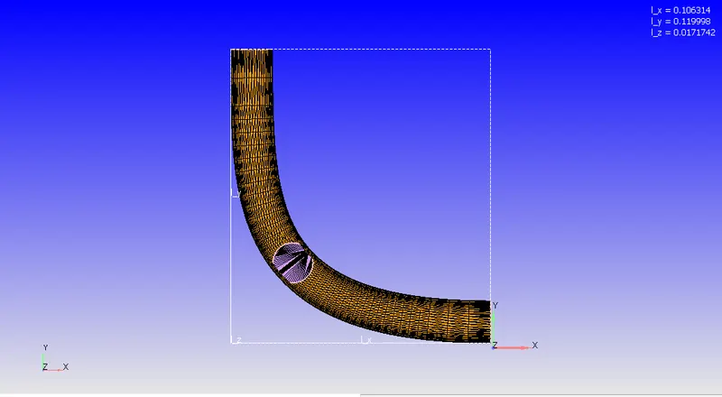
The geometry consists of an elbow pipe of diameter ~0.017m and arc length of the pipe as ~1m. The butterfly valve is modelled by a circular disk which is not connected to the pipe walls is approximately ~0.014m. After loading the STL file and repairing the geometry using CONVERGE Studio's inbuilt functions, we flag the boudaries and provide them with appropriate jargon used by CFD practitioners.

The appropriately boundary flagged geomtery's cut section view is as follows. The geometry clearly highlights the presence of the throattling valve (circular disk) inside the fluid domain (elbow pipe)

Case Setup:

The case setup for for the current study is carried out using the CONVERGE Studio Case Setup GUI. The following settings have been chosen for the simulation in the respective subtree

• Application type subtree:
  • Time-based application is chosen due to the nature of the simulation
• Materials subtree:
  • Pre-defined mixture of standard Air (77% Nitrogen and 23% oxygen by mass fraction) and are considered as non reactive. The gas simulation and global transport parameters are set to default values.
• Simulation parameters subtree:
  • A steady state, compressible solver is chosen. Since the geometry is relavtively simple, we set the simulation type as full hydrodynamic.
  • The starting time/cycle is set to 0 and the total number of cycles for the simulation is set 15000. The max convective CFL number is set to 1 to satisfy the CFL criteria.
  • A steady state monitor for velocity is set at the outlet to check for convergence for a sample of 500 cycles. The relative tolerance and max standard deviation for this project is 0.001.
  • The solver parameters is set to a density based PISO algorithm with default settings for solving the linear systems
• Boundary Conditions subtree:
  • Inlet: Pressure boundary - Total Pressure of 150000 Pa (1.5 bar), velocity boundary - zero normal gradient, Temperature boundary - Fixed Value of 300K, Species boudnary condition: Fixed value of Standard Air, turbulent kinetic energy and dissipation boudnary: default values
  • Outlet: Pressure boundary - Total Pressure of 100000 Pa (1.0 bar), velocity boundary - zero normal gradient , Temperature boundary - Backflow Value of 300K, Species boudnary condition: BackFlow of Standard Air, turbulent kinetic energy and dissipation boudnary: default values
  • Pipe Wall: Pressure boundary - zero gradient , velocity boundary - Law of Wall, Temperature boundary - law of Wall with wall temperature as 300K,turbulent kinetic energy and dissipation boudnary: default values
  • Throttle body: (Full open position) Pressure boundary - zero gradient , velocity boundary - Law of Wall, Temperature boundary - law of Wall with wall temperature as 300K,turbulent kinetic energy and dissipation boudnary: default values
  • Regions and initialization: Doamin is initialized with stationary standard Air at 300K and 1.5 bar and default values of turbulent kinetic energy and turbulent dissipation.
• Physical Models subtree:
  • For the current simulation, we have chosen Renormalized group Reynolds Averaged Navier Stokes (RNG RANS) model with default parameters.
• Grid Control subtree:
  • The base grid settings for cell dimension is set to 0.001m in all directions.
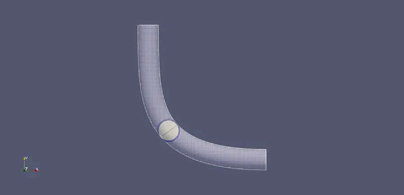
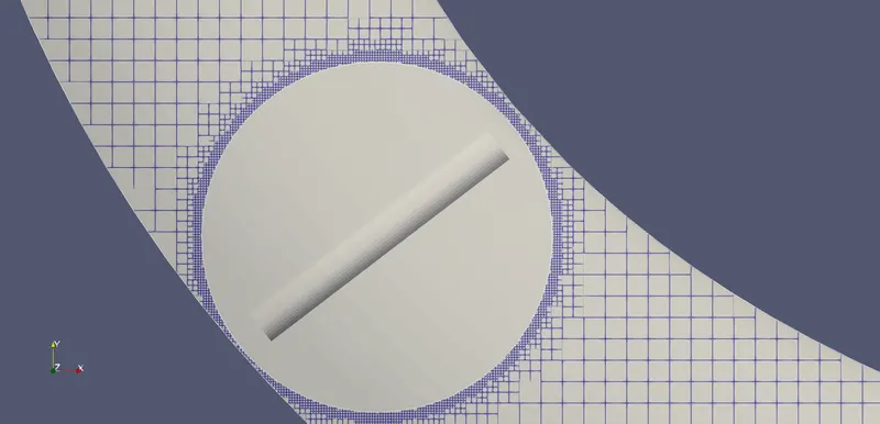
  • A fixed embedding is provided on the throttle body which is permanent. The scale and the embedding layers is set to 3
  • The cut section of the mesh which includes the throttle device and a close up of the embedded layers is illustrated as follows

Simulation Results:

The contours and the line plots generated using Paraview and Converge Studio are as follows

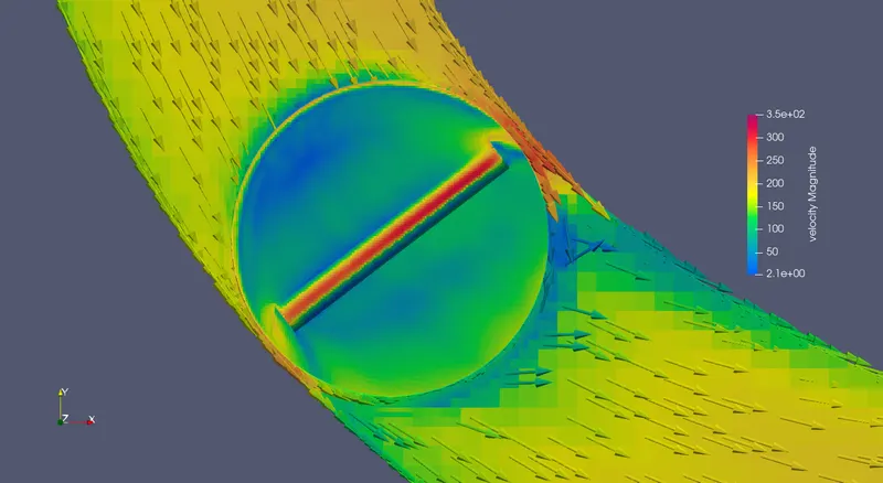
Velocity Contour with vector field:

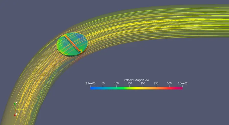
Velocity Contour with streamlines:

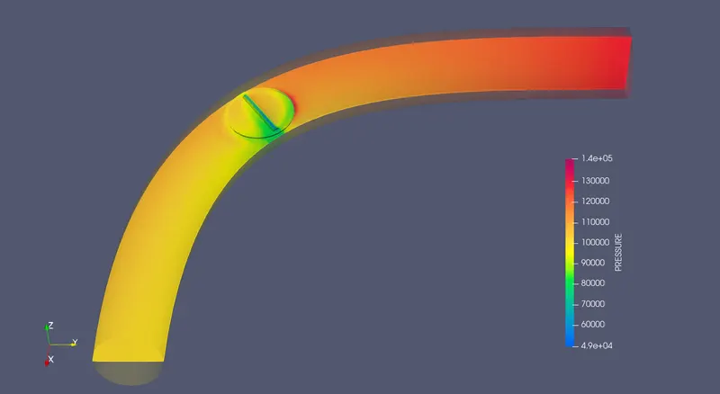
Pressure Contour:

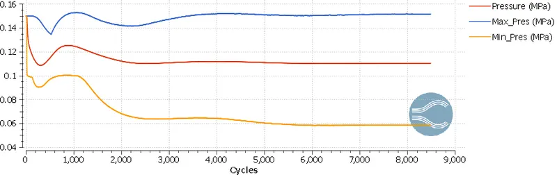
Maximum, Average, Minimum Pressure in the Domain:

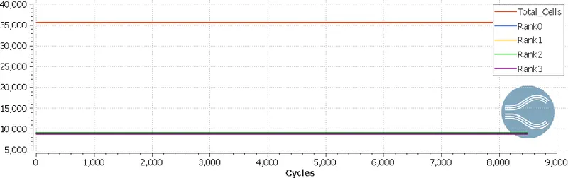
Cell count with cells divided to each processor:

\

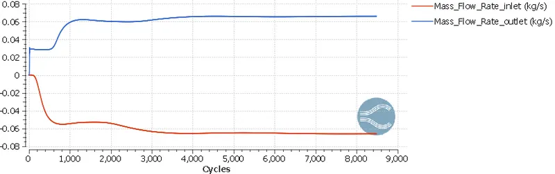
Average Mass flow rate at inlet and outlet:

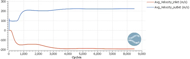
Average Velocity at inlet and outlet:

From the above plots and contour, we note the following observations,

1. From the line plots of flow parameters of velocity, pressure and mass flow rate, we can conclude that the results have reached steady state.
2. From the line plot of cell division, we observe that the load balancing between the four processors have been almost equal.
3. From the pressure and velocity contours, we can get results which are expected i.e. the flow is obstructed minimially due to the fully open position of the throttle valve. The pressure rise is observed where the fluid is halted near the valve and low pressure zones are formed where the fluid accelearates.

Conclusions:

From this simulation, we understood how to accurately capture flow around a body using fixed embedding technqiues. The advanced post processing of the velocity and pressure field for generating interesting contour plots was understood and implemented.