Week 4 - CHT Analysis on Exhaust port

Aim:

Perform CHT Analysis on exhaust port using ANSYS Fluent.

Objectives:

1. Provide brief introduction on the usage, verification of Conjugate Heat Transfer Analysis and its validation with experimental data.
2. Prepare the geometry and generate a mesh for the simulation.
3. Simulate and post-process results obtained from the simulation.
4. Summarise the post-processed results

Introduction:

Conjugate heat transfer analysis is a type of simulation where heat transfer processes in the fluid and solid equations are considered simulatenously for understanding the flow of energy through the computational domain. The conduction heat transfer is mostly dominated in the solids which occurs due to molecular diffusion. On the another hand, convection heat transfer is observed in fluids due to its ability to advect the thermal energy along the flow direction. In simulation software, the heat transfer between the solids and fluids occur by allowing the thermal energy to flow through interface between the two regions. As a result, a fine mesh is required near the interface to properly resolve the temperature distribution around the interface and for accurately calculating heat fluxes and heat transfer coefficients.

The CHT analysis is generally used where fluid interacts with the solid for the purpose of extracting or supplying heat for example heat exchangers such as condensors and evaporatos. In the study of fluid-structure interaction such as temperature hot-spots in the IC Engine cylinder are determined using the CHT analysis and then are used as boundary and initial conditions for the structural analysis.

From the CHT analysis, we obtain various solution parameters such as the temperature, velocity, density and pressure field distribution. Apart from these standard field variables, we also obtain the heat transfer coefficient between the solid and fluid interface. This is an important parameter as it provides critical insight on the performace of devices like the heat exchangers.

We can verify the results of the predicted HTC results of the simulation using the following methods:

• From the definition of the Nusselt Number.
  • We can use turbulence flow correlations such as Dittus-Bolter equation or Sider-Tate equation for calculating the Nusselt Number on the basis of the Reynolds and Prandtl number and then using the thermal conductivity of the fluid, we can obtain the value of the heat transfer coefficient.
• From the definition of the convection heat flux
  • From the theoretical definition of the heat flux, we can obtain the local heat transfer coefficient which depends on the local temperature of the fluid in contact of the solid interface. This provides a much better results compared to the averaged HTC values as they take into consideration the near-wall treatment and local temperature of the fluid.
• From available experimental and theoritical values for simple geometries.

The accuracy of the heat transfer coefficient in simulation depends on several parameters. Here we list few of the important ones:

• Near Wall Treatment (Based on Prandtl number, the temperature boundary layer can be smaller or larger than the momentum boundary layer, thus requiring proper wall functions depending on the mesh resolution)
• Turbulence models
• Physical and theromdynamical properties of the fluids and solids considered
• Number of mesh elements (Ideally should be grid independent. So, through grid dependence study should be carried out for CHT analysis)

In this study, we simulate a multi-inplet exhaust port to observe the effects on the walls of the pipe through which the exhaust gas is travelling. Our objective is to gain a steady state result for the problem which consists of conduction and convection processes.

Geometry:

The geometry of the exhaust port consits of 4 inlets connected to a single outlet via identical pipes. For generating conformal mesh, we need to share the toopolgy and generate a interface between the fluid and solid regions. All these preprocessing is carried out using the ANSYS built-in toolkit SpaceClaim. The pre-processed geometry can be visualized as follows:

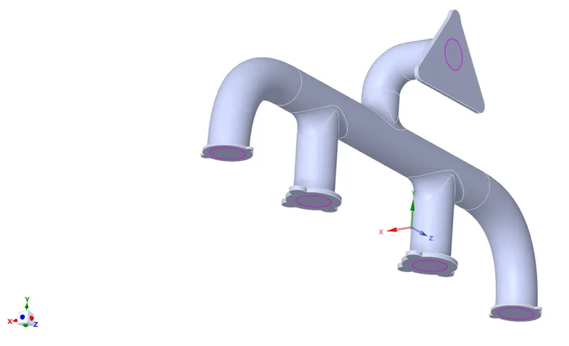
From the above geometry, the purple boundaries present at the inlet and the outlets denote the interface of the shared topology of the fluids and the soilds.

Meshing:

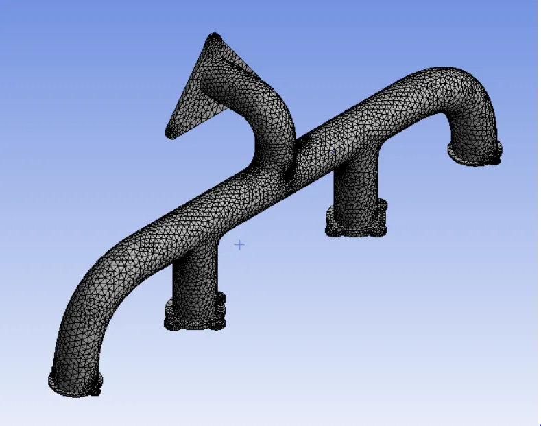
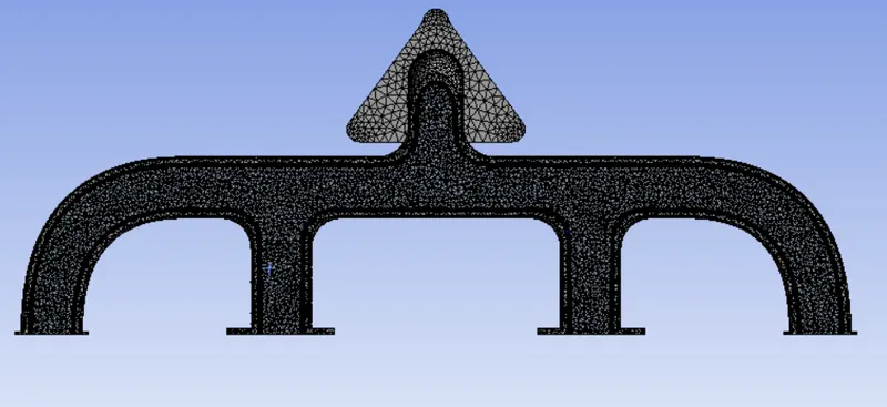
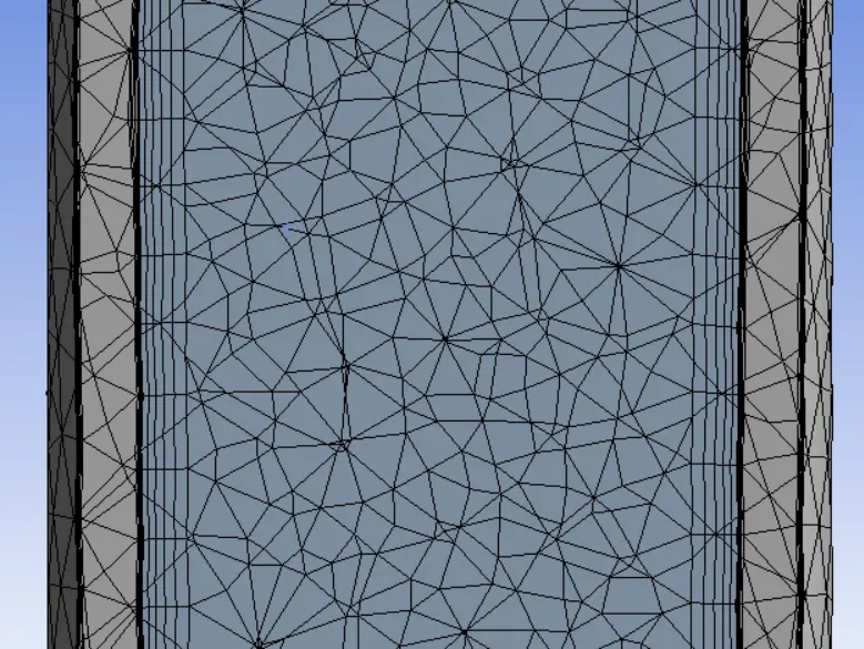
For the current study, two meshes meshes are considered. The first one is the baseline mesh which is generated by using the default settings (element size 0f 0.15 m) and the second is the refined mesh for which inflation layers at the interface and the edge of the pipe-walls are considered for better prediction of the heat transfer coefficients. The element size of the fluid domain for the refined mesh is 0.1 m and 5 inflation layers of 0.01 m total thickness on the interface and pipe walls. We will call the baseline mesh as mesh 1 and the refined mesh as mesh 2 for the rest of the study. The meshes defined above are visualized as follows

Mesh 1

Cut section view of Mesh 2

Close up view of the Mesh 2 interface

Case Setup:

For both cases, identical simulation settings are chosen. The simulation settings used for both the simulations are as follows:

• General
  • A pressure-based, steady state solver is chosen as the Mach number for the simulation is < 0.3 and we are only interested in the final state of the simulation which is independent of the initial conditions.
• Models
  • As the inflation layers are made such that the first cell layer thickness is in the log-law region, we utilize the reliazable k-`epsi` model.
  • To ensure that all the near wall treatment of the boundary near the interface is done using the log-law region, we utilize the scalable wall functions for the near wall treatment.
• Materials
  • The workinfg fluid is chosen as air and the working solid is chosen as aluminium.
  • The thermodynamical and physical properties are chosen from the Fluent database.
• Boundary conditions
  • Inlets: All inlets allow the flow of air into the domain at 5m/s normal to the boundary and temperature of 700 K.
  • Outlet: Outlet boundary condition at zero gauge pressures
  • Pipe walls: Convective boundary condition with a heat transfer coefficient of 10 W/m^2 K and free stream temperature at 300 K
  • Remaining walls: Walls with adiabatic boundary conditions
• Initialization
  
  • We intialize the domain with velocity calculated using the hybrid boundary conditions
• Calcualtion activities
  • To observe the distribution of the temperature on the walls of the pipe, an animation is setup to plot the temperature contours after 10 iterations of the steady state solvers.
• Run Calculations
  • The simulation ran for 500 iterations where the temperature contours are observed to reach a steady state.

Simulation Results:

Mesh 1

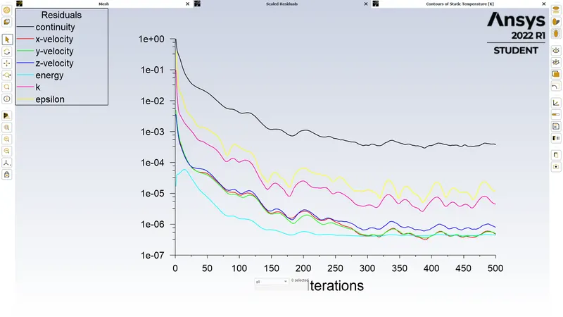
• Residuals vs number of iterations

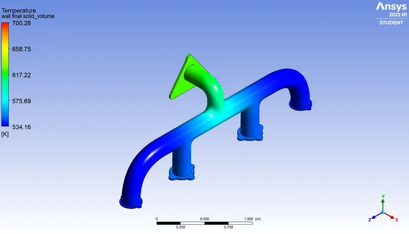
• Temperature Contours of the pipe wall

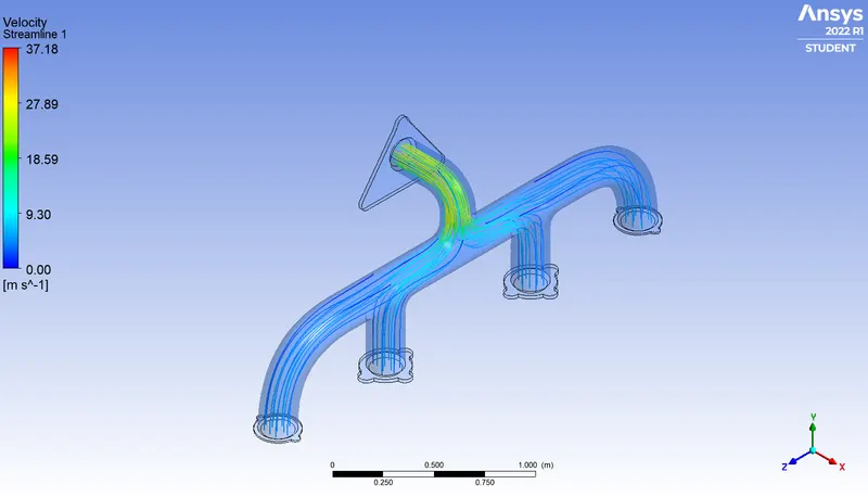
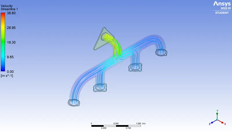
• Streamline plots of velocity from inlets to outlets

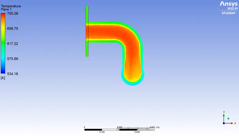
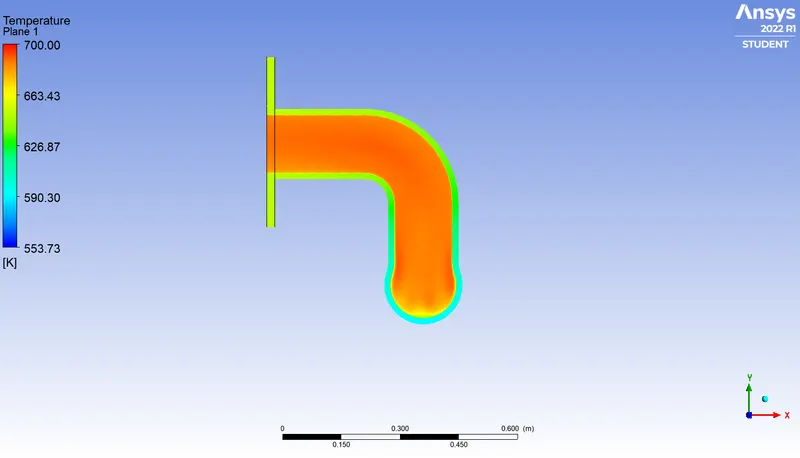
• Temperature contour in the XY Plane

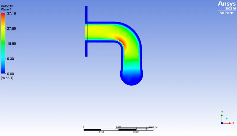
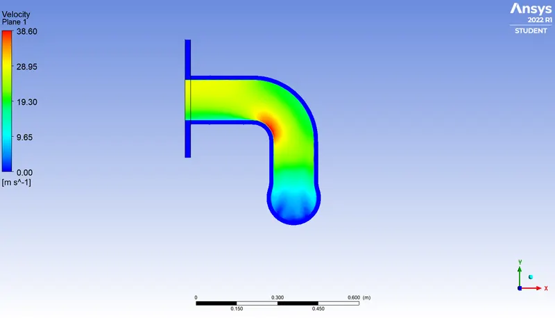
• Velocity contour in the XY Plane

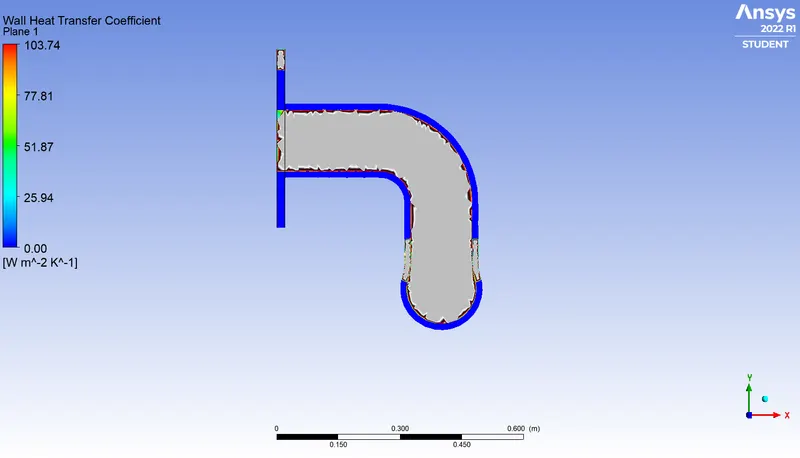
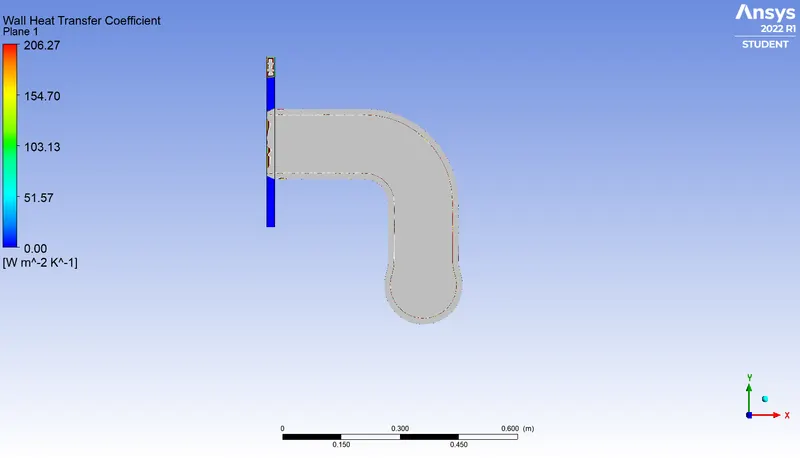
• Wall Heat Transfer Coefficients contour in the XY Plane

Mesh 2

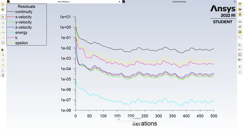
• Residuals vs number of iterations

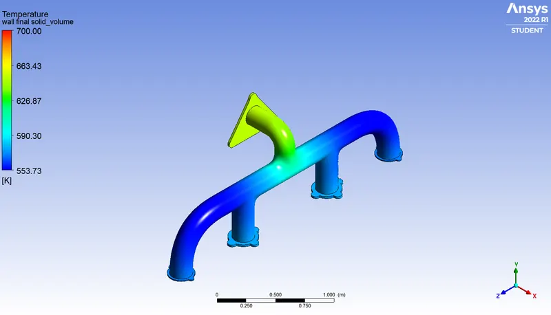
• Temperature Contours of the pipe wall

• Streamline plots of velocity from inlets to outlets

• Temperature contour in the XY Plane

• Velocity contour in the XY Plane

• Wall Heat Transfer Coefficients contour in the XY Plane

Conclusions:

1. The residuals in both cases have a oscillatory behavior and hence can not provide information regarding the convergence to steady state for the current study.
2. The temperature contours on the pipe walls reach steady state and are identical for both the cases.
3. From the stream lines we observe that because of mass conservation the fluid velocity accelerates near the outlet of the exhaust port.
4. From theory, it is expected that convective heat tranfer is proportinal to the local velocity of the fluid. This is observed for both the cases where heat transfer coefficient is maximum where the fluid velocity is maximum in the domain.
5. The baseline case provides faster results but the accuracy of the results are questionable due to improper refinement near the interface. The effects are visible on the heat transfer coefficients of both cases.