Week 3: Flow over a backward facing step

Aim:

To understand the effect of meshing step size on the simulation of backward facing step using CONVERGE.

Governing Equations:

The air flow in the backward facing step simulation is modelled by the compressible Navier-Stokes Equations which consists the continuity, momentum and energy conservations and the transport of the oxygen and nitrogen species in the air is modelled by convective diffusive equations.

These partial differential equations are derived by applying conservation laws on differential control volume. For brevity, we skip the long and contrived derivations of these laws and recommend the reader to refer the comprehensive Wiki articles for fiurther detail.

Objectives:

• Describe the important theory of the flow features of the backward step geometry
• Generate 3 meshes for the backward facing step geometry using CONVERGE Studio
• Record the case setup for the simulation in CONVERGE Studio
• Visualise the simulation results by making line plots, contours and animation of the flow features in CONVERGE Studio and Paraview

Theory:

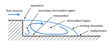
The backward facing step is a simple two dimensional geometry which is characterized by the sudden expansion of the cross-section, appearing as a step pointing in the direction opposite to the general flow.

The sudden expansion causes a adverse pressure gradient which detaches the boudnary layer from the wall causing flow separation. The flow between the separated boudnary layer and the bottom and side walls forms a recirculation region, whose shape and vorticity strength depends on the geometry (expansion ratio) and the flow parameters such as the velocity and pressure. The separated flow reattaches to the bottom wall after travelling a certain distance which is called as the reattachement length. This problem acts as simplified model of the seperating flows observed in the nature and industrial applications. For CFD practitioners, this geometry provides an ideal platform to test turbulence models since it depicts all the essential features of the seperated flows with relatively simple geometry structure.

As a result, this problem has become an important benchmarking case in the field of the turbulence modelling. An simplified illustration of the backward facing step with all the important flow features is as follows:

Geometry:

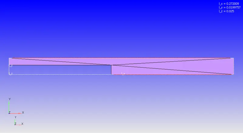
Since the geometry shape is fairly basic, it was natively generated using CONVERGE Studio's limited CAD capacity. After checking diagnostics and flagging all the boundaries, we proceed to case setup. The geometry generated along with its dimensions in meters is visualized as follows:

Case Setup:

The simualtion settings were done through the CONVERGE Studio Case Setup GUI.

The application was chosen as Time-Based under the application type subtree.

The working fluid was chosen as standard Air (77% Nitrogen and 23% Oxygen by mass fraction) in the Materials subtree. The fluid is assued to be non-reactive for the simulation. The default gas simulation parameters and global transport were used for the current study.

In the run parameters subtree, we chose a steady state, compressible solver and set the simulation at 'full hydrodynamic' because of the relatively simple geometry. For steady state stopping criteria, we choose to monitor the average temperature, average density and average velocity at the outlet sampled for 500 cycles for a relative tolerance of 0.001 for all the aformetioned parameters. The total number of iterations/cycles is set to 15000, with the maximum convective Courant Number set to 0.5 for satisfying the CFL criteria. The fluid flow solver is chosen as density based PISO algorithm with default parameters since it has been reportedly proven in literature that PISO has a superior performance over SIMPLE algorithm for the backward facing step simulation.

In the boundary subtree, the boudnary flags marked on the fluid domain are assigned the following boundaries:

• Inlet: Total pressure = 101525 Pa, velocity = zero gradient, Standard Air at 300K and default values of turbulent kinetic energy (k) and turbulent dissipation(`\epsilon`)
• Outlet: Static pressure = 101325 Pa, velocity = backflow with Standard Air at 300K and default values of turbulent kinetic energy (k) and turbulent dissipation(`\epsilon`)
• Walls: Law of the wall for temperature and velocity, zero gradient of the turbulent kinetic energy and wall model for the turbulent dissipation
• Front and Back: Set to two-dimensional. This makes the geometry a slice of an infinte backward face step geometry

The domain is initialized to Standard Air at 300K and 101525 Pa with zero velocity in all directions and default values of turbulent kinetic energy (k) and turbulent dissipation(`\epsilon`) in the initial conditions and events subtree.

The Renormalized group k-`\epsilon` (RNG RANS) model with default semi-empirical constants was used for the current simulation.

Mesh Generation:

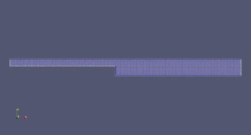
In the current study, we generate three meshes with fixed embedding of scale and embedded layers both set to 1. The embedding will aid us to resolve the complex flow phenomenon occuring near the walls of the domain.

Mesh 1: `dx = dy = dz = 2 times 10^{-3}`

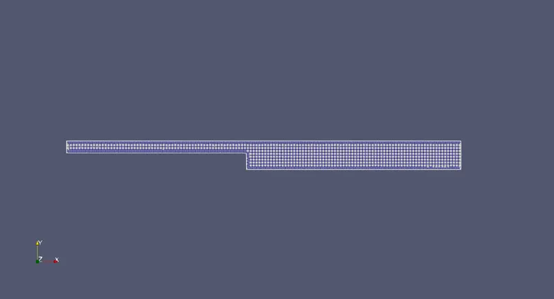
Mesh 2: `dx = dy = dz = 1.5 times 10^{-3}`

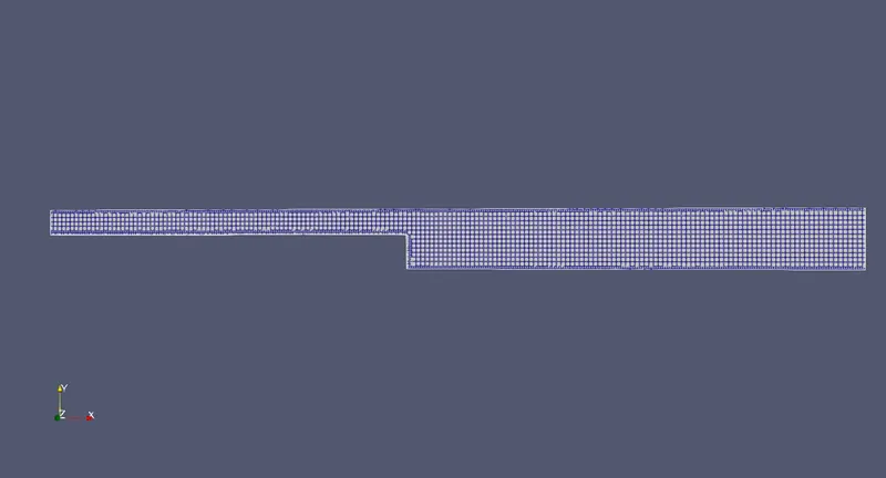
Mesh 3: `dx = dy = dz = 1 times 10^{-3}`

Simulation Results:

Mesh 1:

Animation:

Mesh 1 Animation

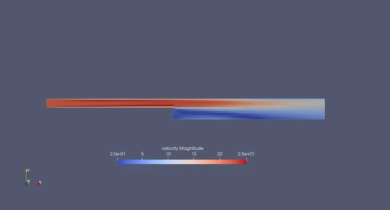
Velocity Contour:

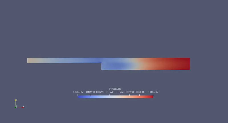
Pressure Contour:

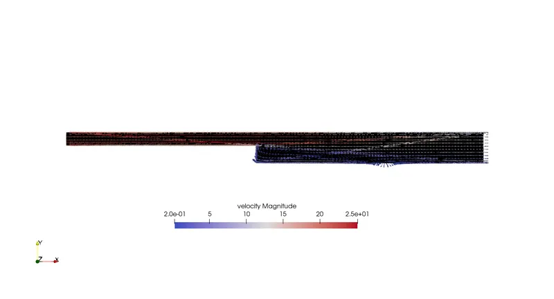
Velocity vector field:

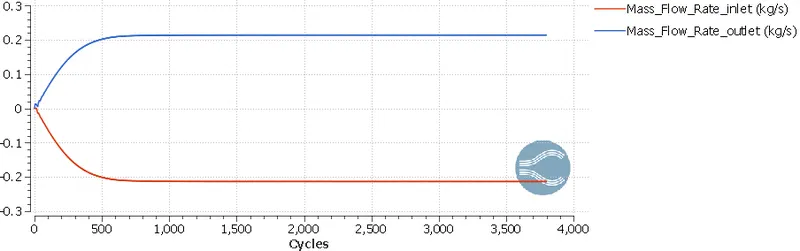
Average Mass Flow rate at inlet and outlet v/s number of cycles:

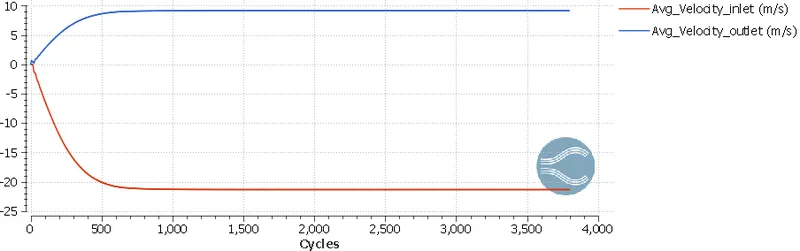
Average Velocity at inlet and outlet v/s number of cycles:

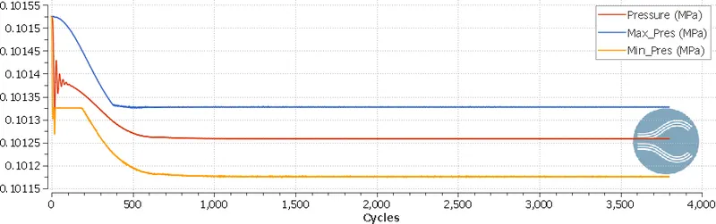
Maximum, mean and minimum pressure in the domain v/s number of cycles:

Cell Count and number of cells to each processor v/s number of cycles:

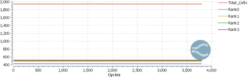
From the above plots and contours, we note the following observations:

1. The velocity and pressure contours are inline with the theoritical expectations (sudden expansion should create an adverse pressure gradient and separated flow, which are observed in the contours)
2. The velocity vector field shows the recircualtion region but the secondary recirculation region is not captured
3. The line plots of the flow parameters (Average velocity, average mass flow rate and max, min and mean pressure) shows no fluctuations. This indicates that the flow parameters have converged but the results might be more diffusive and hence less accurate.

Mesh 2:

Animation:

Mesh 2 Animation

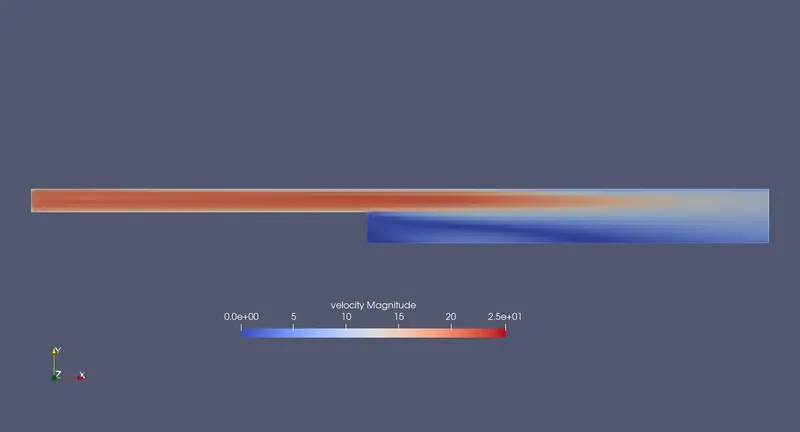
Velocity Contour:

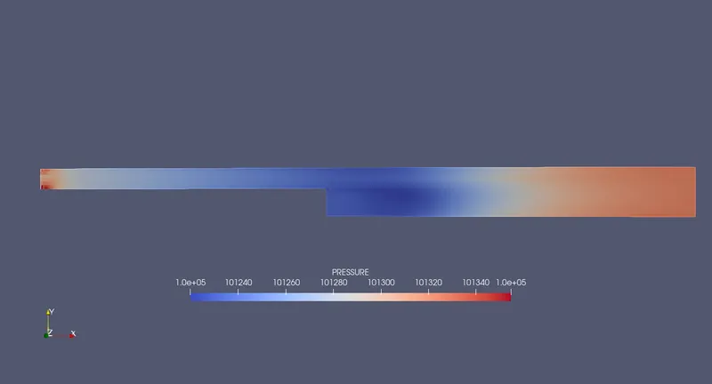
Pressure Contour:

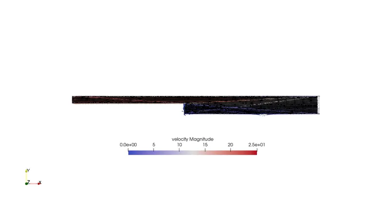
Velocity vector field:

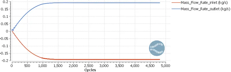
Average Mass Flow rate at inlet and outlet v/s number of cycles:

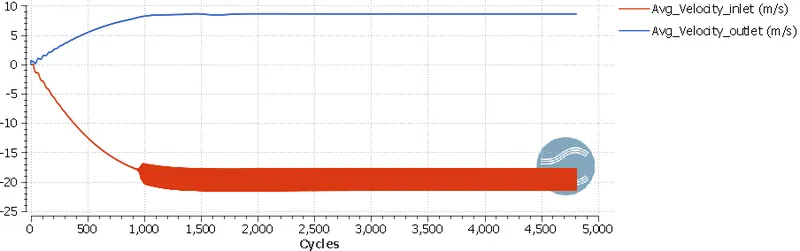
Average Velocity at inlet and outlet v/s number of cycles:

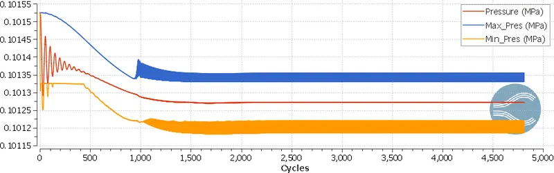
Maximum, mean and minimum pressure in the domain v/s number of cycles:

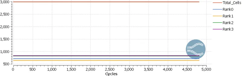
Cell Count and number of cells to each processor v/s number of cycles:

From the above plots and contours, we note the following observations:

1. Similar to Mesh 1, the overall flow development in Mesh 2 is inline with the theoritical expectation
2. The velocity vector field shows the recircualtion region and secondary recircualtion region, which depicts the higher accuarcy of Mesh 2
3. The line plots of the flow parameters show considerable flucations around the mean values. This indicates that flow parameters are signifcantly dependent on mesh, which decreases the reliablity of the results.

Mesh 3:

Animation:

Mesh 3 animation

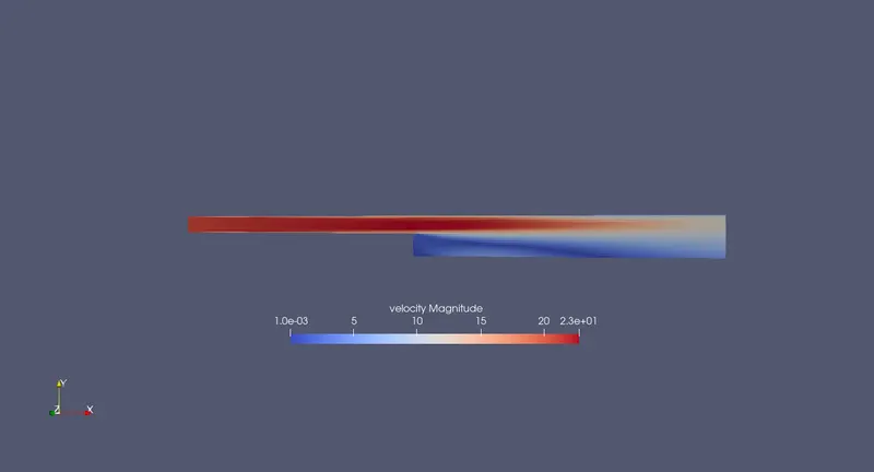
Velocity Contour:

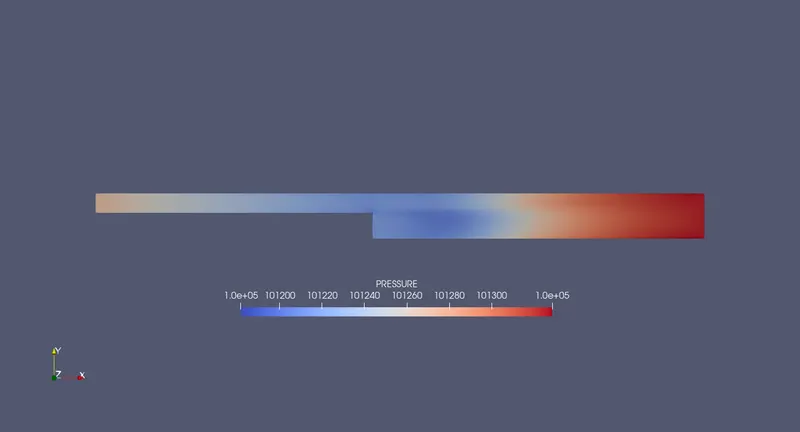
Pressure Contour:

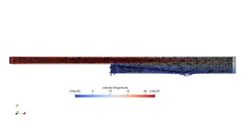
Velocity vector field:

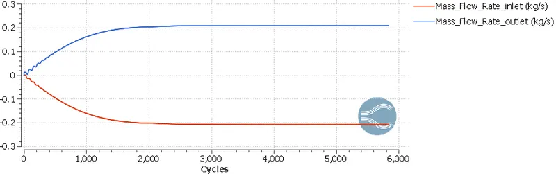
Average Mass Flow rate at inlet and outlet v/s number of cycles:

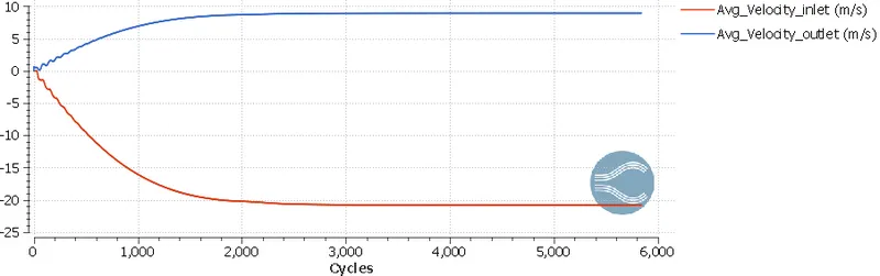
Average Velocity at inlet and outlet v/s number of cycles:

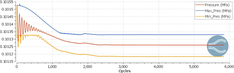
Maximum, mean and minimum pressure in the domain v/s number of cycles:

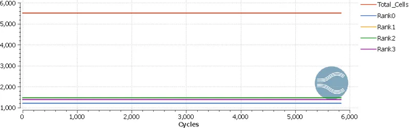
Cell Count and number of cells to each processor v/s number of cycles:

From the above plots and contours, we note the following observations:

1. Similar to Mesh 1 and Mesh 2, the overall flow evolution using Mesh 3 is inline with the theoritical expectations.
2. The velocity vector field shows the recircualtion region and secondary recircualtion region,similar to Mesh 2.
3. The line plots of the flow parameters show no flucations around the mean values. This indicates that flow parameters are converged and are accurate due to the fine nature of Mesh 3.

Conclusion:

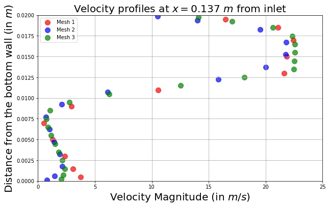
From the above simulations, we understood how to make a relatively primitive geometrical body like backward facing step in CONVERGE Studio to perform a mesh dependence study. The velocity profile of the three meshes are compared in the following image