Week 1: Channel flow simulation using CONVERGE CFD

Aim:

To understand the preprocessing, simulation, and post-processing workflow in CONVERGE by simulating flow through a channel.

Governing Equations:

For the simulation, we use the steady state, compressible Navier-Stokes equations to model the flow of the air and non-reacting convective diffusive equation to model the species of nitrogen and oxygen present in the air.

Navier-Stokes Equations:

Mass: `nabla . (rho vec U) = 0`

Momentum :`nabla (rho vec U otimes vec U ) = - nabla p + nabla . tau`

Convective-Diffusive Eqaution for species concentration:

`nabla .( D nabla c) = nabla . (vec U c)`

The Navier Stokes equation is derived by applying Newton's Second Law of motion on a fluid particle. In the steady state formulation, the temporal variation of the velocity is set to null. The transport equation for species concentration is the result of application of Renyolds Transport Theorem for species conservation in a bounded domain. The symbols used in the above equations have their standard meanings and any interested reader should refer to the respective Wiki articles for further details.

Objectives:

1. Generating and visualizing 3 meshes for the channel geometry using CONVERGE Studio.
2. Simulating the fluid flow for all the meshes using CONVERGE.
3. Visualizing and explaning the pressure and velocity contour in Paraview.
4. Visualizing and explaning the pressure, velocity, mass flow rate and total cell count plots in CONVERGE Studio.
5. Animating the flow evolution from the initial to the converged state in Paraview.

Geometry:

The channel geometry is built in the CONVERGE Studio using the box shape function. The length of the box along the x direction is 0.1 m (which is the flow direction) and 0.01 m in the y and z directions.

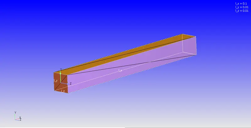
The geometry which is defined by the traingles are assigned to the following named boundary conditions: inlet, outlet, top and bottom walls and front and back boundaries. The normal direction are corrected by using the transform function.

Case Setup:

Using the Converge Studio GUI, we select the application type as Time-Based solver. In the Materials subtree, we choose the predefined mixture of air as our working fluid for the simulation and non-reacting species of nitrogen and oxygen are selected for the species file.

In the Run parameters subtree, we select the steady state solver with full hydrodynamic as the simualtion mode for capturing the appropriate flow physics. A steady state monitor is set to start after 500 iterations to identify whether the steady state is already reached before total number of iterations. This is an important feature as it reduces the computational resources usage. The flow features monitored are Average Velocity, Average Density, Average Temperature at the outlet boundary and the Nitrogen and Oxygen species mass fraction in the fluid domain. The convergence is checked by averaging the results from 100 iterations and checking whether they satisfy the tolerance range for the mean and range for the standard deviation which is both set to 0.01 in our simulation.

The total number of iterations are set to 15000 with minimum time step of 1e-9 and maximum time step of 1. In the solver parameters, we choose a density based PISO solver for Navier-Stokes eqaution with the convection courant number set to 0.5 as per the CFL criteria.

We assign all the boundaries to the fluid domain region. The boudnary condition values are set as follows:

• For the inflow condition, we set the total pressure as (1.0001 bar) 100010 Pa, zero gradient condition for the velocity, 300K as the temperature boudnary condition and standard air as the species boundary conditon.
• For the outflow condition, we set the static pressure as (1 bar) 100000 Pa, a backflow boundary conditon for the velocity with standard air as the species boundary and 300K as the temperature boundary.
• For the top and bottom walls, we provide a stationary no-slip walls and fixed value of 300K for temperature.
• The front and the back boundary are provided the 2D boundary condition, such that the problem is only solved in the x and the y direction.

The fluid domain is initialized with the 0 velocity in all direction, temperature as 300K and pressure value set as 100010 Pa. The oxygen mass fraction is set 0.77 while the nitrogen mass fraction is set to 0.23 (The steady state results should be relatively independent of the initial conditions)

The simualtion is laminar as a result no turbulence model is chosen. The varaibles such as the pressure, density, velocity, temperature and mass fraction of the nitrogen and oxygen are selected for post processing. The writing time interval for the files is kept as 50 while the writing interval for restart files is set as 100.

Mesh Generation:

Mesh 1: The dimensions of the cell for the mesh are `dx = 2.0e-04`, `dy = 2.0e-04` and `dz = 2.0e-04`. The total number of mesh cells in this mesh is 25000.

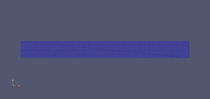
Mesh 2: The dimensions of the cell for the mesh are `dx = 1.5e-04`, `dy = 1.5e-04` and `dz = 1.5e-04`. The number of mesh cells in this mesh is ~45000.

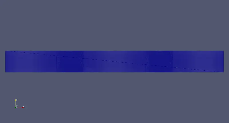
Mesh 3: The dimensions of the cell for the mesh are `dx = 1.0e-04`, `dy = 1.0e-04` and `dz = 1.0e-04`. The number of mesh cells in this mesh is 100000.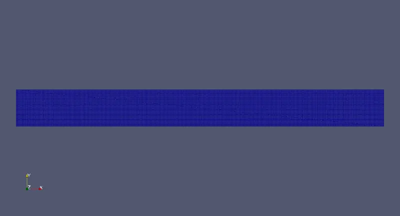

Simulation Results:

The contours and the plots from the three simualtions are listed as follows:

Mesh 1:

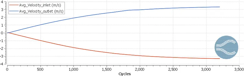
Average Velocity at inlet and outlet vs number of iterations

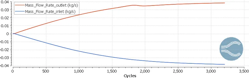
Average Mass Flow Rate at inlet and outlet vs number of iterations

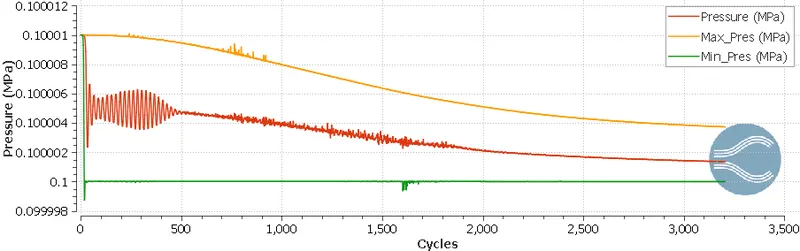
Maximum, Average and Minimum Pressure vs number of iterations

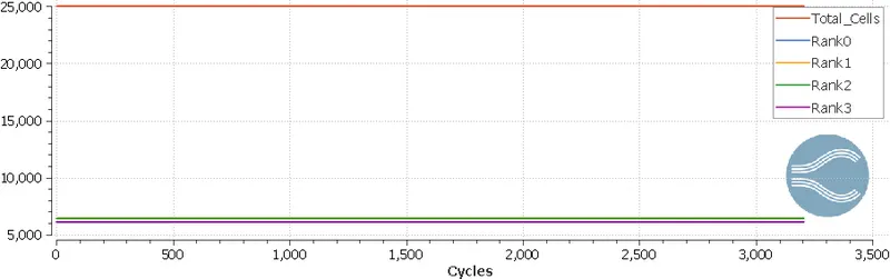
Cell Count and Cell for each processor vs number of iterations

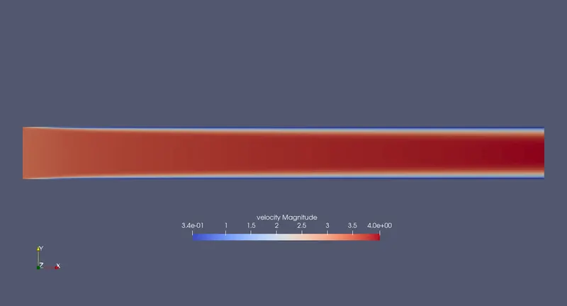
Velocity contour at the last iteration

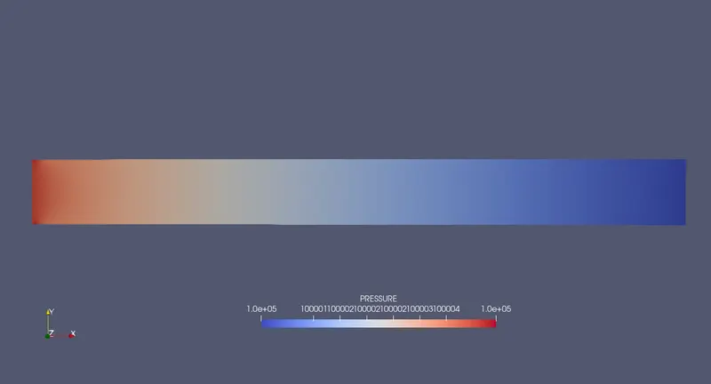
Pressure Contour at the last iteration

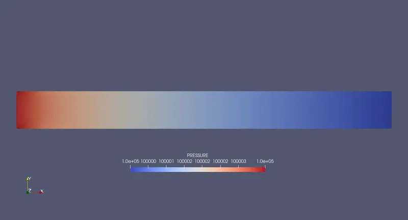
For Mesh 1, we note the following observations:

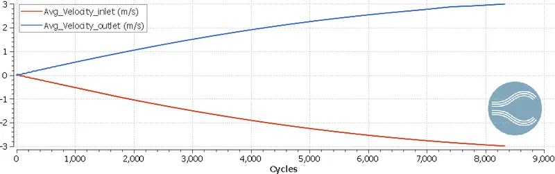
1. From the plots that the averaged value of the velocity and mass flow rate at the inlet and the outlet are equal, which is inline with the theory of conservation of mass
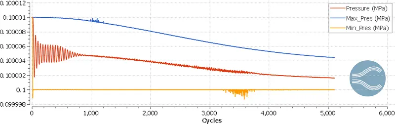
2. The maximum, average and minimum pressure are smaller than the total pressure, which provides a basic validation for our results.
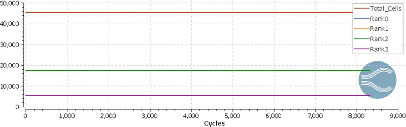
3. From the cell count plot, we observe that the total number of cells are 25000 and the cells are almost equally divided between the 4 processors
4. The pressure and velocity contours are inline with theoritical result of the channel flow

Mesh 2:

Average Velocity at inlet and outlet vs number of iterations

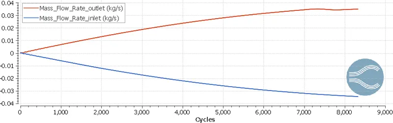
Average Mass Flow Rate at inlet and outlet vs number of iterations

Maximum, Average and Minimum Pressure vs number of iterations

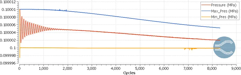
Cell Count and Cell for each processor vs number of iterations

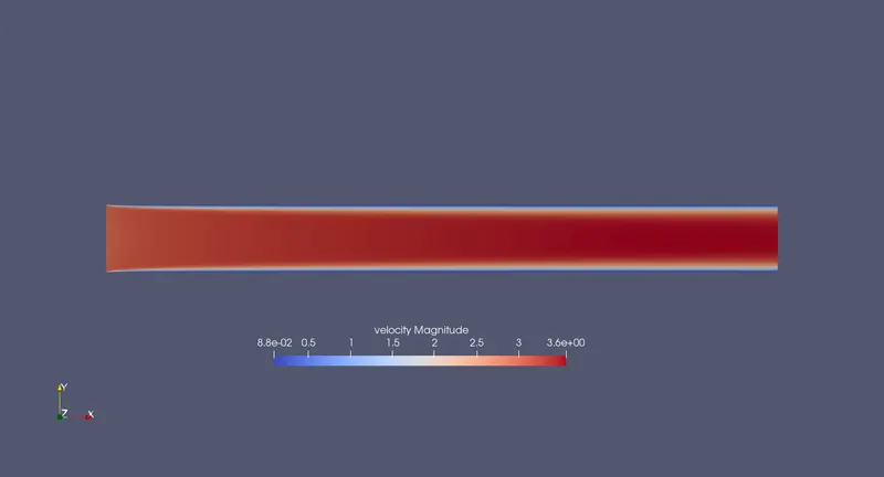
Velocity contour at the last iteration

Pressure Contour at the last iteration

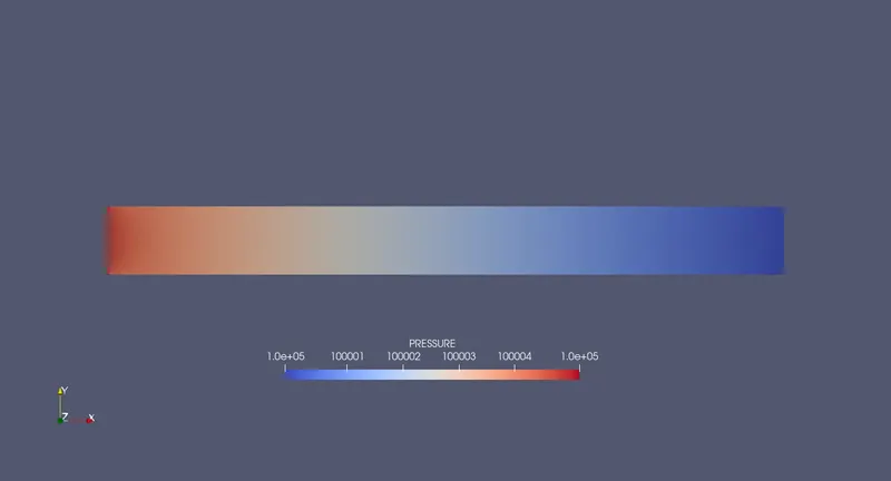
For Mesh 2, we note the following observations:

1. The average velocity, mass flow rate and pressure plots are similar to that observed for Mesh 1. Hence, the results of this mesh are also accurate
2. The cells in the processors are not equally divided and hence the solution takes a longer amount of time to converge because of the cell count imbalance, which was observed in this simulation
3. The pressure and velocity contours are inline with the theoritical results of the channel flow

Mesh 3:

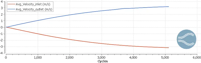
Average Velocity at inlet and outlet vs number of iterations

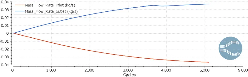
Average Mass Flow Rate at inlet and outlet vs number of iterations

Maximum, Average and Minimum Pressure vs number of iterations

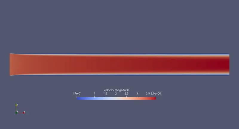
Velocity contour at the last iteration

Pressure Contour at the last iteration

For Mesh 3, we note the following observations

1. The average velocity and mass flow rate at the inlet and outlet for all iterations are balanced, similar to the previous meshes, hence the results are appropriate.
2. The total number of cells are 100000 and are almost equally divided for the four processors, hence the simualtions converge quickly compared to the previous mesh
3. The velocity and pressure contours are inline with the theoritical results of the channel flow.

Mesh Comparision:

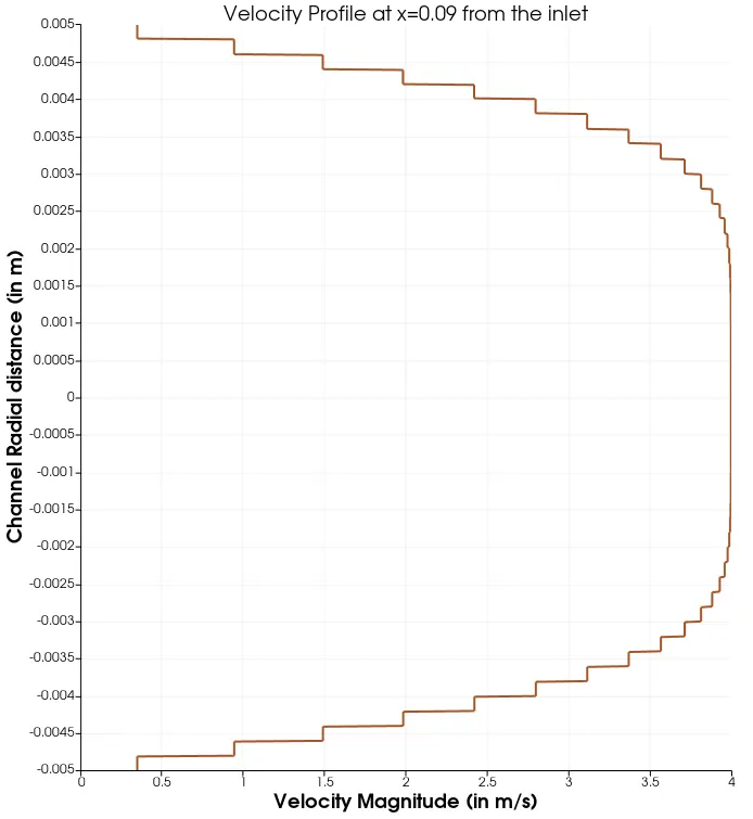
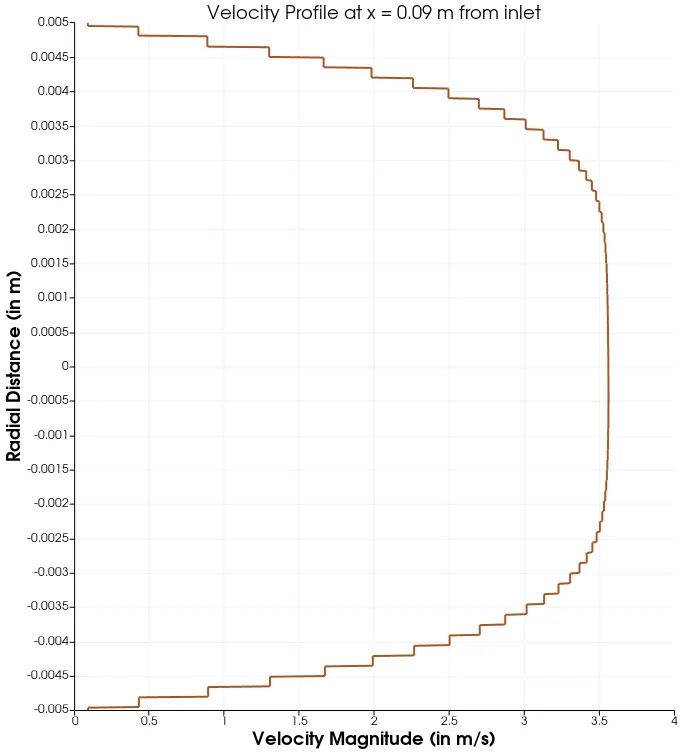
We compare the performance of the three meshes by plotting the parabolic fully developed velocity profile near to the outlet of the channel. The results are as follows:

Mesh 1:

Mesh 2:

Mesh 3:

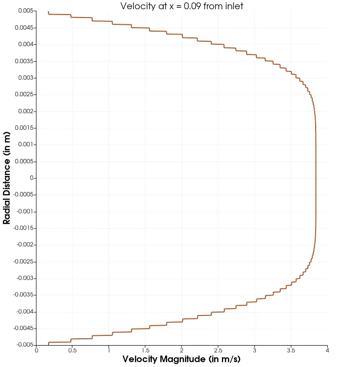
From the above plots, we can conclude that the all three meshes accurately calculates the velocity profile as per the theoritical values and the profile gets more precisce with increasing the number of cells.

Conclusions:

By simulating the channel flow, we have developed a standardized workflow for pre-processing, simualting and post-processing in CONVERGE which will be essential for working on complex projects.