Week 1- Mixing Tee

Aim:

Perform a comprehensive simulation study of the mixing-tee geometry using ANSYS Fluent.

Objectives:

1. Preparing the fluid domain from the mixing-tee CAD geometry.
2. Generating mesh for the fluid domain and carrying out a mesh dependence study.
3. Choosing the appropriate turbulence model by performing a comparison study between k-`omega` and k-`epsi` models.
4. Performing steady-state simulations and post-processing results to study the effect of the length of the geometry and the momentum ratio.

Preparing the fluid domain:

The fluid domain is generated using the ANSYS Fluent's native CAD generation tool called as SpaceClaim. The mixing-tee geometry was generated in SolidWorks and imported into SpaceClaim. After importing the geometry, we can visualize it as follows:

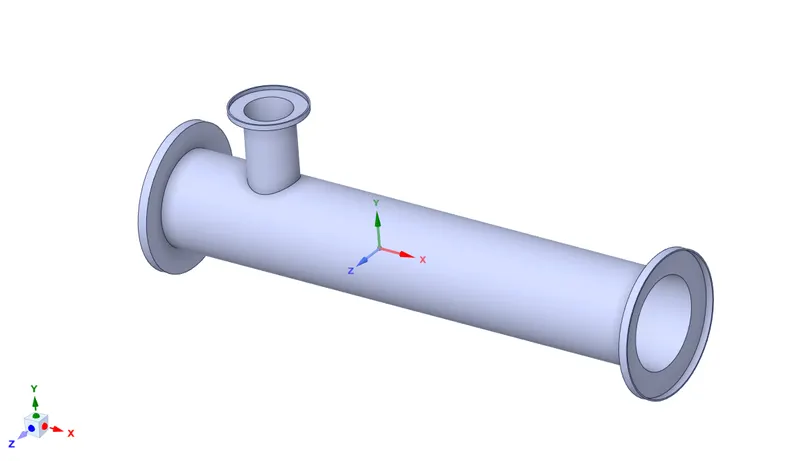
From the above figure we can observe that the geomtry has solid regions with non-zero thickness (for instance: annular pipe walls). These regions are included in analysis only when we are intrested in the temperature distribution in the walls of the pipe and such analysis can be performed using Conjugate Heat Transfer.

In the current study, our focus is only on the mixing of the two fluids at different temperatures, hence we can remove the solid regions from the analysis without sacrificing any accuracy. The process of extraction is carried out by using the "Volume Extract" feature in Space Claim. The edges which bound the volume are selected and the volume is extracted. After this process, we hide the solid domain and use the feature "suppress for physics" to ignore it for the futher analysis. The extracted domain is visualized as follows:

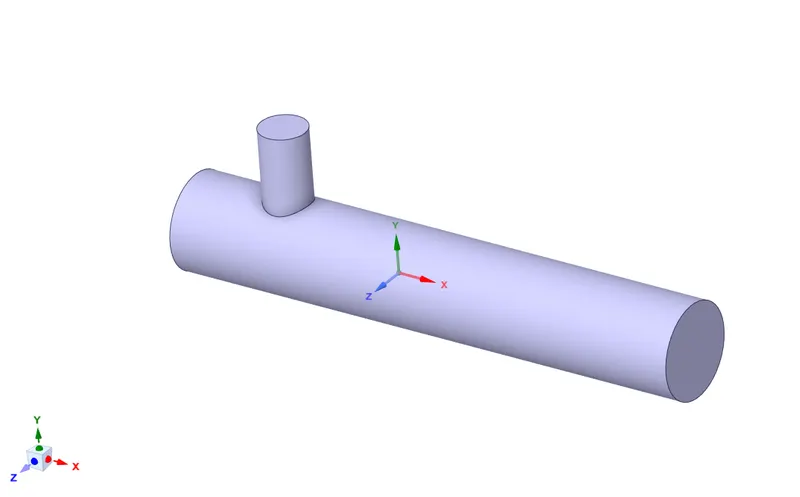
From the above figure, we can conclude that the fluid domain is successfully extracted. The above process was carried out for the "short" mixing-tee geometry. The same steps are used for the "long" mixing-tee geometry and hence the details are skipped here for the sake of brevity.

Meshing:

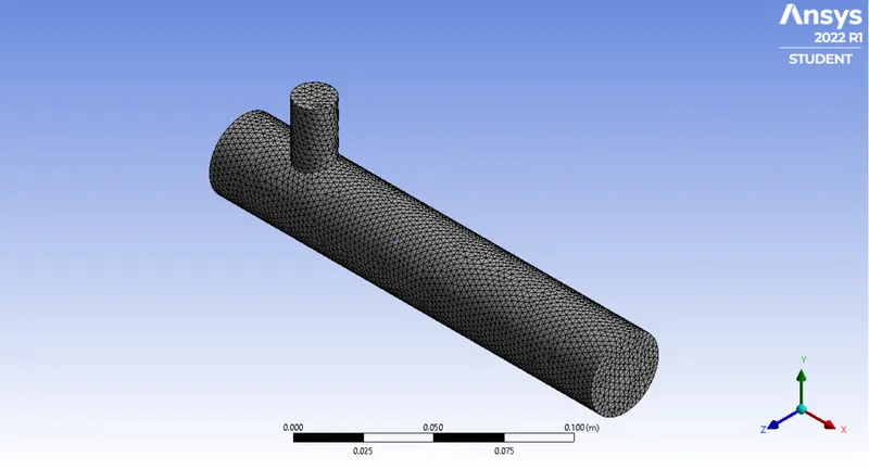
We use the inbuilt tool in ANSYS Workbench for meshing the fluid domain and this tool is called as Mesher. The Mesher tool automatically generates a mesh with default parameters which are determined from the bounding box of the domain. For carrying out the mesh dependence study, we provide different values of the element size. The elements size chosen for the current study are: `10^{-2},\ 7.5 times 10^{-3},\ 5 times 10^{-3} and 2.5 times 10^{-3}\ m`. For the comparison study between the turbulence models, we use the coarse mesh of `10^{-2}\ m`. The different meshes are visualized as follows

Coarse mesh: `10^{-2}\ m`

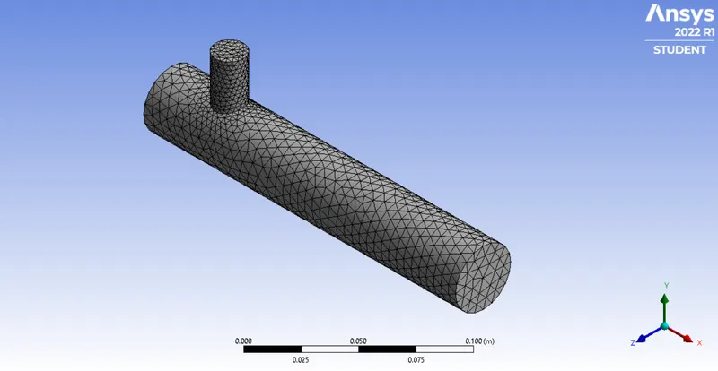
Intermediate Mesh: `7.5 times 10^{-3}\ m`

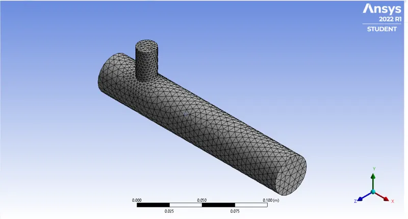
Fine Mesh: `5 times 10^{-3}\ m`

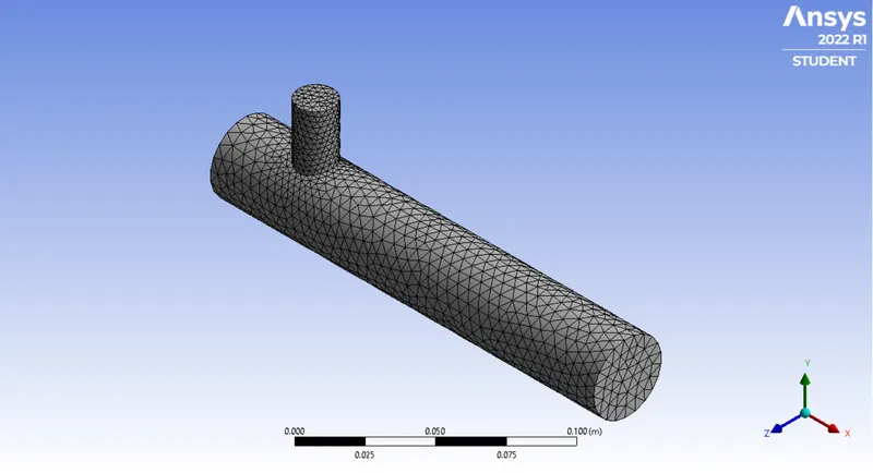
Finer Mesh: `2.5 times 10^{-3}\ m`

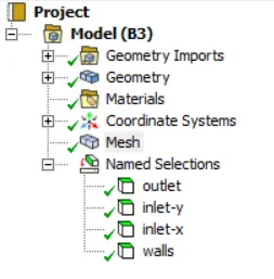
After performing the meshing, we provide appropriate names to the boundaries. This is a great practice as we will see during the setup of the simulation, the solver can identify the type of the boundary from the name string of the boundary. We provide the following descriptivenames for all the meshes for easy identification when providing the boundary conditions.

Setting up the case:

After providing appropriate boundary names and generating mesh, we setup the simulation case and run the simulation using the Fluent. We setup the all the cases in the current study with the following settings:

• General
  • Since the Mach number in the simulation will be lower than 0.3, we use a pressure based solver.
  • The simulation type is steady state solver and the velocity formulation is absolute.
• Models
  • Since the current simulation deals with mixing of two fluids at different temperature we consider the energy equation while solving the Navier-Stokes equation.
  • For the turbulence modeling, we will perform a comparison study between the k-`omega` and k-`epsi` models and appropriate model is chosen when performing the simulation.
• Materials
  • The working fluid is air and its thermodynamical and physical data for the fluid is determined from ANSYS material database.
• Cell Zone Conditions
  • We validate that the working fluid chosen in the Materials section is appropriately selected in the interior of the fluid domain.
• Boundary Conditions
  • Because of our appropriate naming of the boundary surface, Fluent can automatically detect the type of the boundary condition.
  • The velocity inlet at the higher temperature has a fixed inlet temperature of 36 deg C and inlet velocity of 3 m/s. The cold inlet has fixed inlet temperature of 19 deg C and inlet velocity dependent on the momentum ratio
  • At the outlet, the gauge pressure is set to zero and at the walls, standard stationary, fixed wall conditions are provided.
• Methods
  • For the current study, we use the default settings for the pressure velocity coupling and spatial discretization available with the turbulence model.
• Controls
  • Similar to the Methods, we use the default settings for the pseudo time explicit relaxation factors.
• Report Definitions
  • Since our objective for the current study is to evaluate the quality of the mixing of the fluids, we make special report of the mean and the standard deviation of the temperature at the outlet.
• Initializations
  • Hybrid intialization is used to provide the intial values for the pressure and velocity. We use 20 iterations of the initializations to reach the tolerance value of `10^{-6}`.
• Run Calculations
  • We run the simulations for 300 iterations for all the cases.

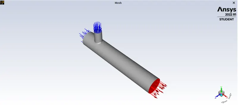
ANSYS Fluent provides a visualization of the simulation with appropriate vectors assigned to the inlets and outlets. The visualization for the current study is as follows:

Selecting the turbulence model:

In this section, we will perform a comparison study for selecting the appropriate turbulence model for the rest of the study. For this study, we use the "short" mixing-tee geometry, coarse mesh and mometum ratio set to 4.

The case setup for both the models is almost identical except in Physical Model section for one case use the Realizable k-`epsi` model with standard wall functions while for the second case we chose the k-`omega` SST turbulence model. We will refer the k-`epsi` model as Model 1 and k-`omega` model as Model 2 from this point. The Workbench provides a nice visualization of the similarity of the two cases.

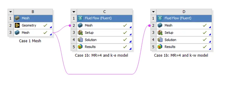
We compare the residuals of the conservation equations, mean and standard deviation of the temperature and contour plots of temperature and velocity for the both the models.

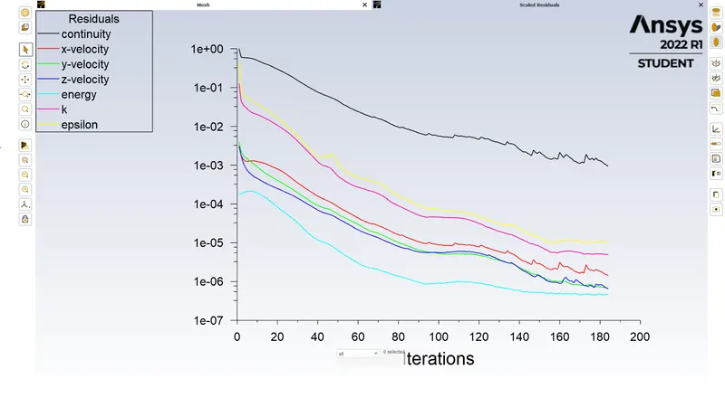
Model 1 Residuals:

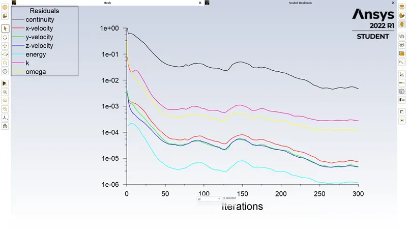
Model 2 residuals:

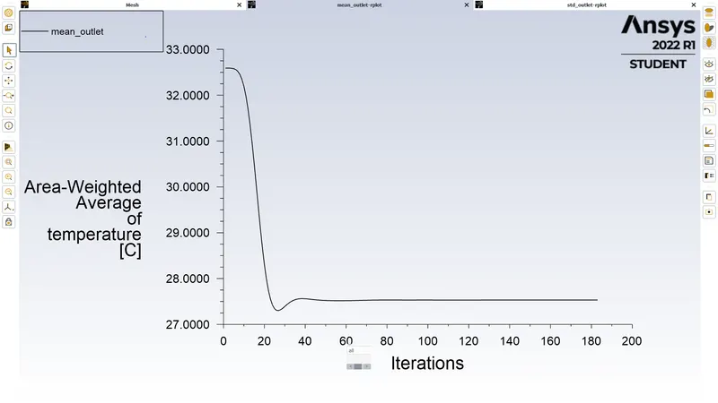
Model 1 Mean of temperature at outlet:

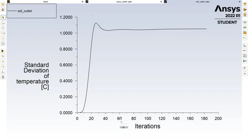
Model 1 standard deviation of temperature at outlet:

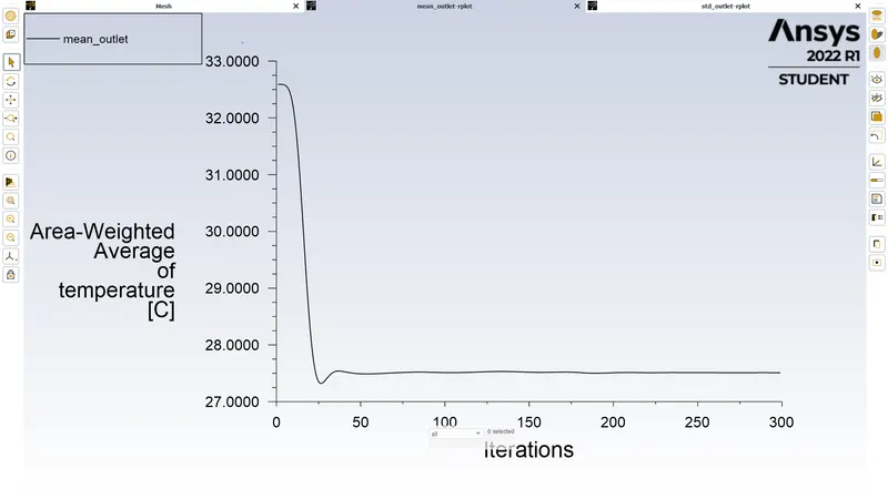
Model 2 Mean of temperature at outlet:

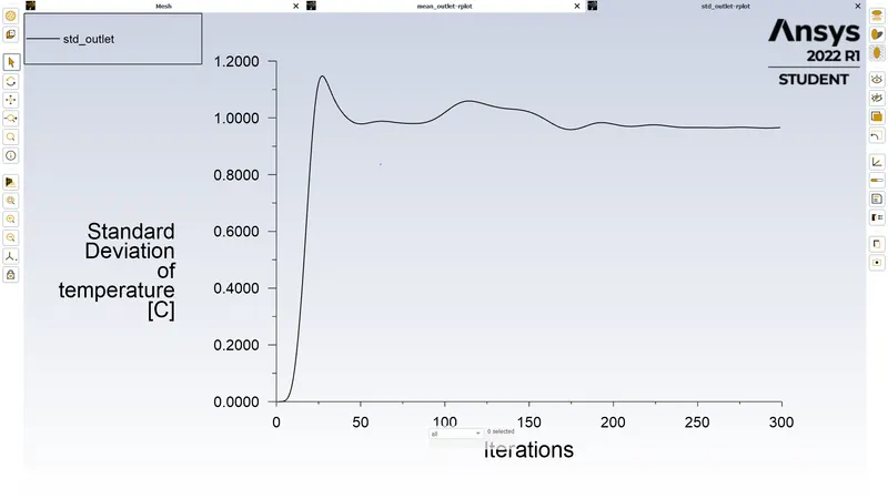
Model 2 standard deviation of temperature at outlet:

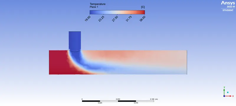
Model 1 temperature contour:

Model 1 velocity contour:

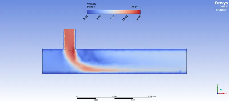
Model 2 temperature contour:

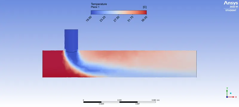
Model 2 velocity contour:

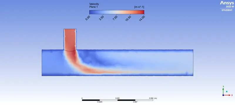
From the above figures of contours and line plots, we note the following observations:

1. The model 1 results are converge at ~180 iterations while the model 2 results are not converged even after 300 iterations.
2. The mean temperature at the outlet is virtually identical for both the models.
3. The standard deviation of the temperature at the outlet has converged for the model 1 while the line plot shows significant variations for model 2.
4. The temperature and the velocity contours look identical for both the models.

If we recall the theory and the use cases for the turbulence models, the k-`epsi` models are used for flows in the shear free region, i.e flow away from the walls while the k-`omega` models are used for flow near to the walls. As a result, the flow near the wall is modelled using wall functions for the k-`epsi` model and on the other hand flow is resolved near the walls in the k-`omega` model.

For the current study, we observe that we are interested in the bulk flow phenomena i.e. mixing of fluids at different temperature and no complex flow phenomenon such as adverse pressure gradients are observed close to the walls. Hence, from these observations, we can safetly choose k-`epsi` model for rest of the study.

Mesh Dependence study:

We carry out the mesh dependence study for the "short" mixing-tee geometry and momentum ratio =4 for the four meshes shown in the Meshing section. To compare the four meshes, we measure the mean and standard deviation of the temperature at outlet of the geometry. We summarise the results of the mesh dependence study in the following table.

Mesh	Mean of T (C)	Relative Error (%)	Std Deviation of T (C)	Relative error (%)
Coarse	27.533	-	1.053	-
Intermediate	27.530	0.01	1.143	8.53
Fine	27.603	0.27	1.281	12.07
Finer	27.533	0.25	1.053	17.79

From the above table, we can conclude that Intermediate mesh will provide results with reasonable accuracy. For the rest of the study, we will use the Intermediate mesh for the simulations.

Effects of Momentum ratio and Length of geometry:

We divide the study into two cases: Case 1 is the "short" mixing-tee geometry and Case 2 is the "long" mixing-tee geometry. Each case consists of two momentum ratios which is denoted as "a" and "b". This parameteric study will help us to quantify the effect of the momentum ratio and the length of the geometry.

The meshing and case setup is identical to those explained in the above sections. In this section, we will skip those details and only report the simulation results obtained from the Fluent solver for brevity.

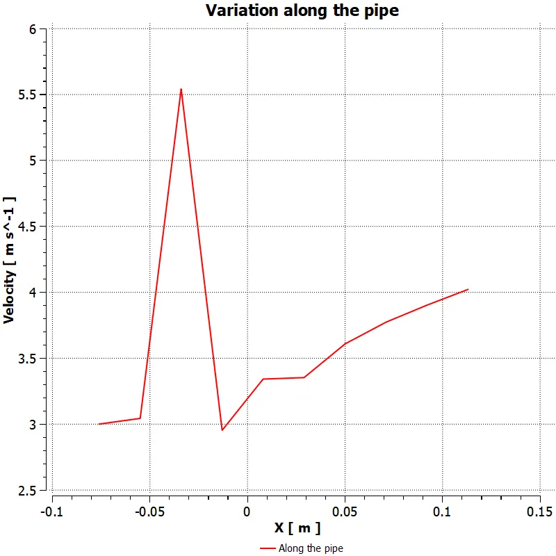
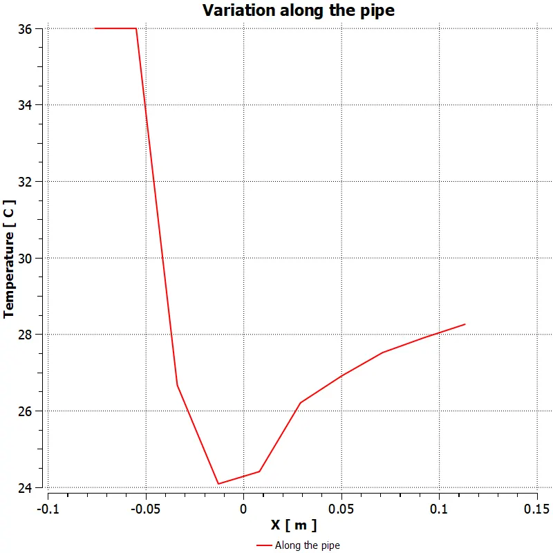
Case 1a:

• Residuals

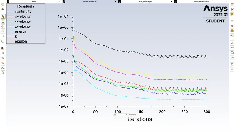
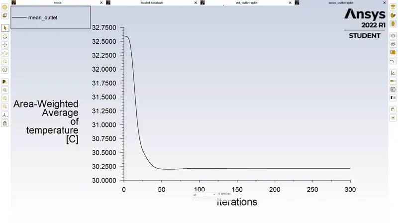
• Mean temperature at outlet

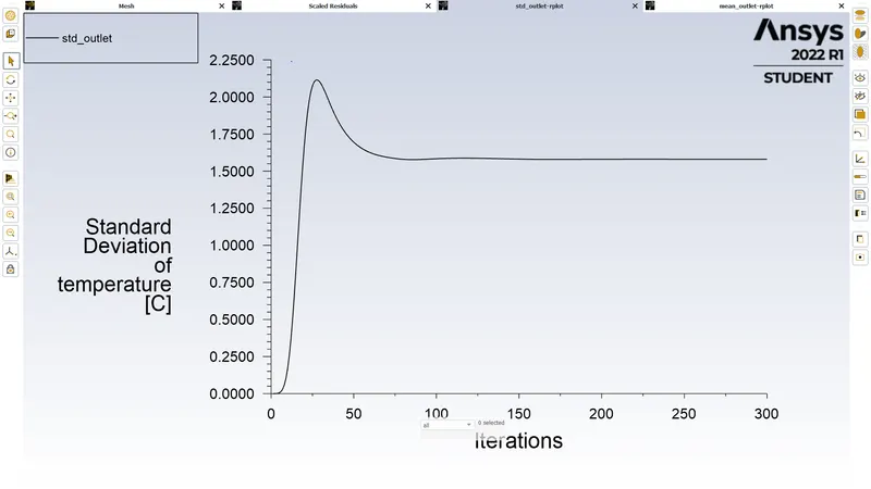
• Standard deviation of temperature at outlet

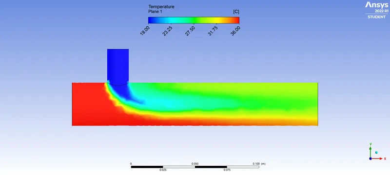
• Temperature contour

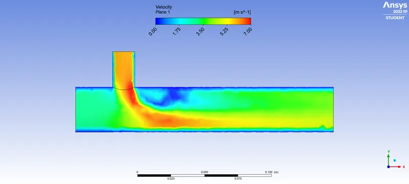
• Velocity contour

• Velocity line plot along the pipe

• Temperature line plot along the pipe

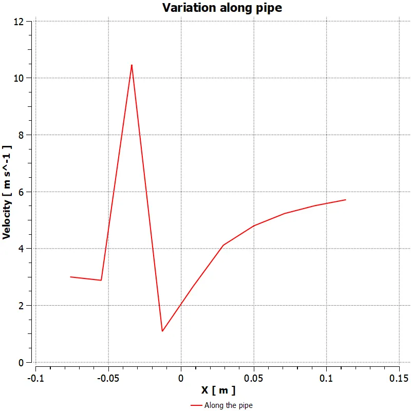
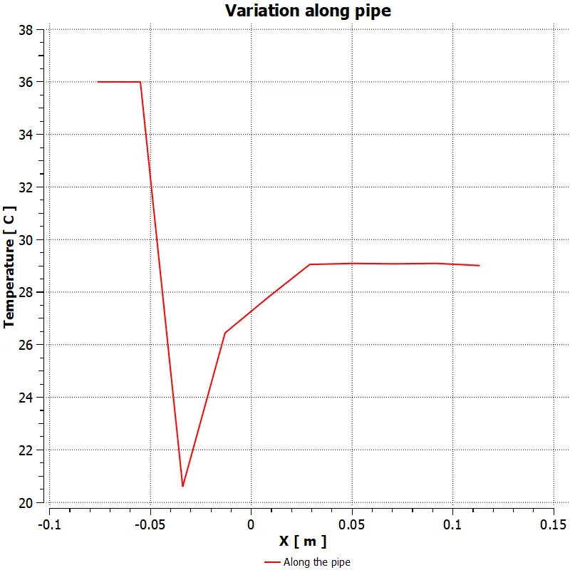
Case 1b:

• Residuals

• Mean temperature at outlet

• Standard deviation of temperature at outlet

• Temperature contour

• Velocity contour

• Velocity line plot along the pipe

• 

• Temperature line plot along the pipe

Case 2a:

• Residuals

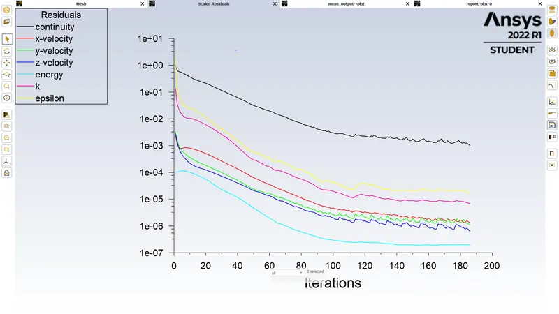
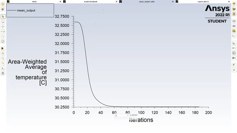
• Mean temperature at outlet

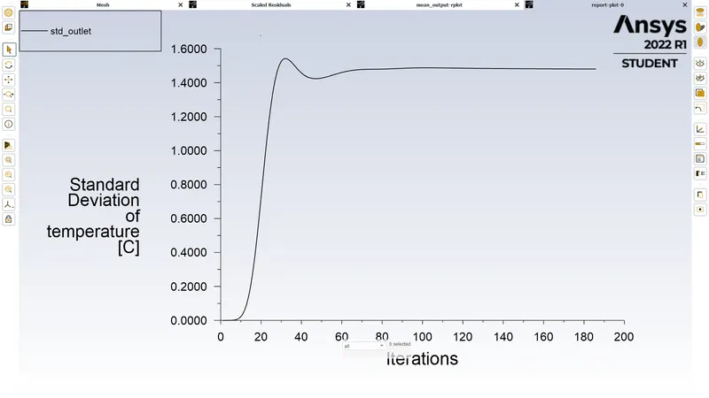
• Standard deviation of temperature at outlet

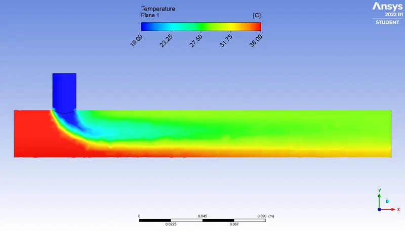
• Temperature contour

• Velocity contour

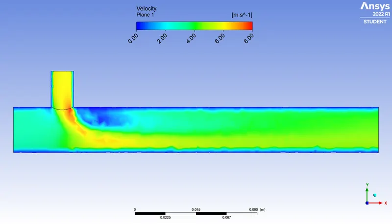
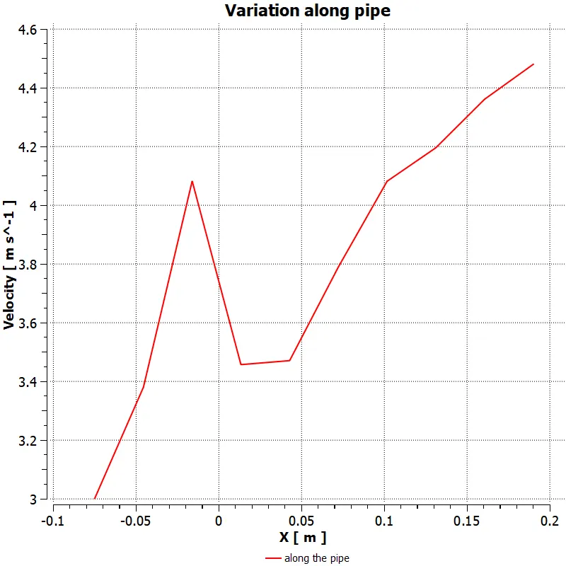
• Velocity line plot along the pipe

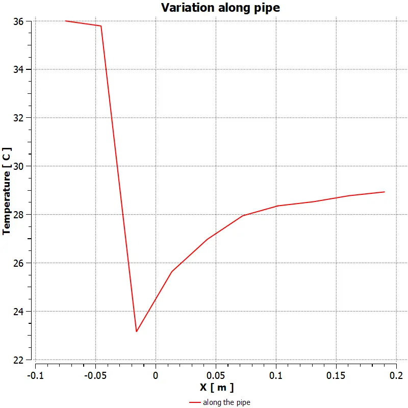
• Pressure line plot along the pipe

Case 2b:

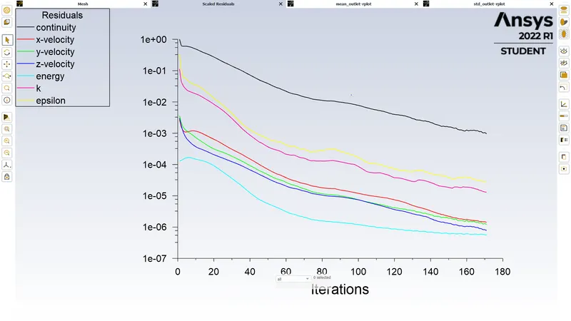
• Residuals:

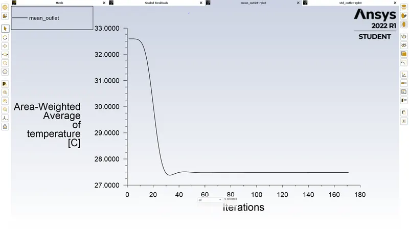
• Mean temperature at outlet

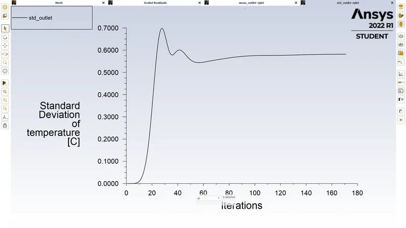
• Standard deviation of temperature at outlet

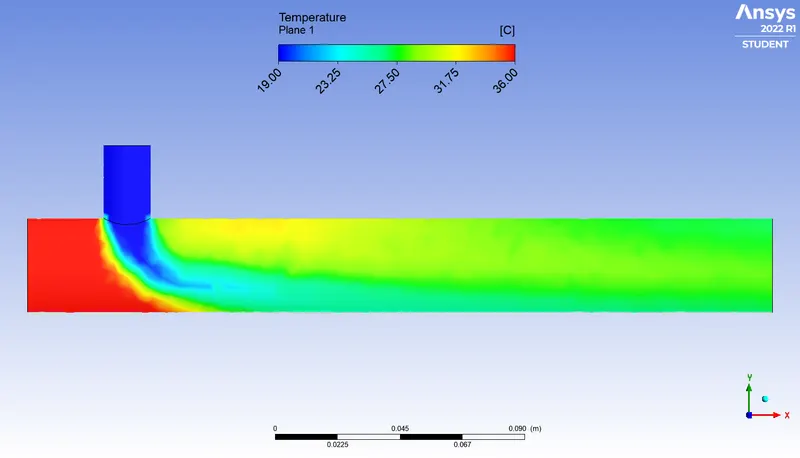
• Temperature contour

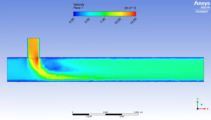
• Velocity contour

• Velocity line plot along the pipe

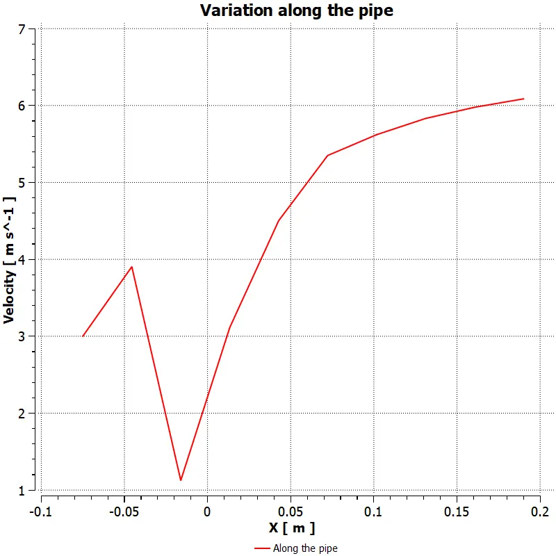
• Temperature line plot along the pipe

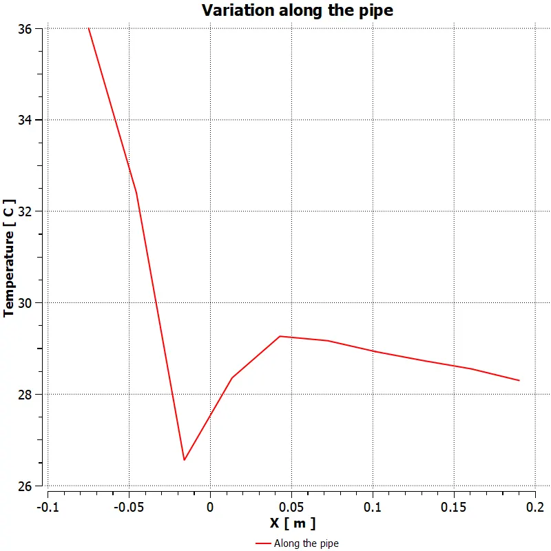
We summarize the results of the 4 cases in a table below:

Mesh	Average Outlet Temp (C)	Cell Count	Number of iterations
Case 1a	30.22	12697	300
Case 1b	27.530	12697	183
Case 2a	30.26	15530	186
Case 2b	27.48	15530	171

From the above results and table we can conclude the following statements.

1. Momentum ratio has a significant effect on the outlet temperature as it promotes turbulent mixing.
2. Length of the geometry has virtually no effect on the outlet temperature because only diffusion is increased which is not very effective in mixing of temperature.