Week 7 - Simulation of a 1D Super-sonic nozzle flow simulation using Macormack Method
Aim:
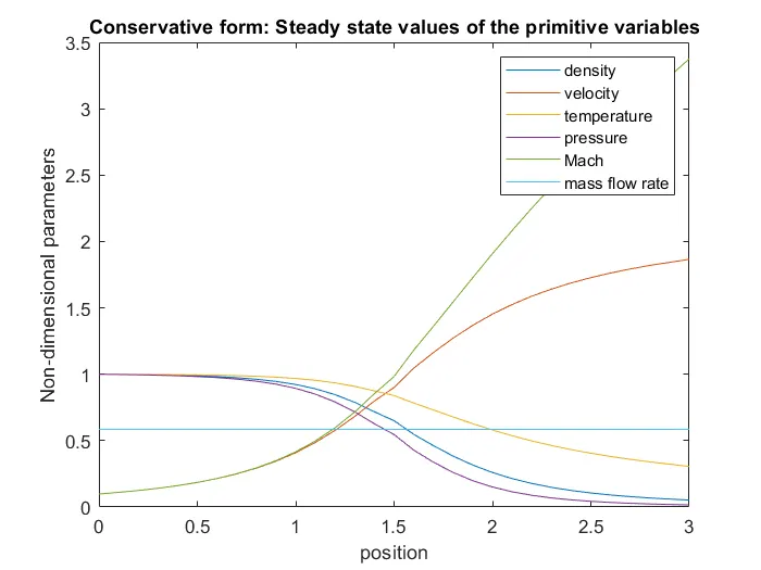
To simulate the isentropic flow through a quasi one-dimensional converging-diverging nozzle using the MacCormack's technique and comparing the steady state results with the exact solution.
The MacCormack method can be used to solve both the conservative and non-conservative governing equations. We will implement both the techniques and compare the quality of the steady state solution obtained from the simulations. We also also carry out grid independence study to determine the optimal number of the grid points required to simulate the flow.
Theory:
The flow through the converging-diverging nozzle is used for generating supersonic flow (Mach number >1) at the outlet from subsonic flow (Mach Number <1) at the inlet due to extreme pressure differences. This flow phenomena is two-dimensional but using some engineering approximations and control volume analysis, we can derive the quasi 1D governing PDE's. These governing equations can be represented as non-conservative (the governing equations are expressed in primitive variables) and conservative (the governing equations are expressed in forms of conserved quantites and fluxes), and both are equivalent in physical sense.
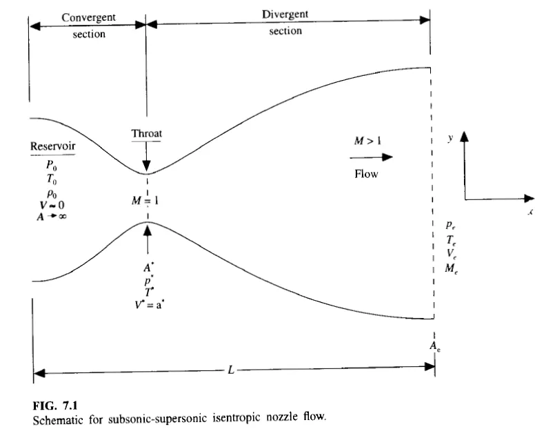
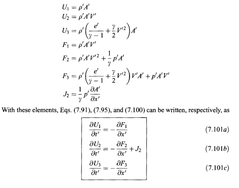
The non-dimensional form of the conservative and non-conservative forms are as follows
Conservative form:
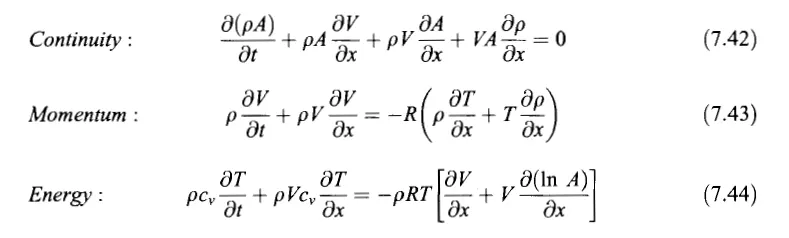
Non-conservative form:
Grid Independence:
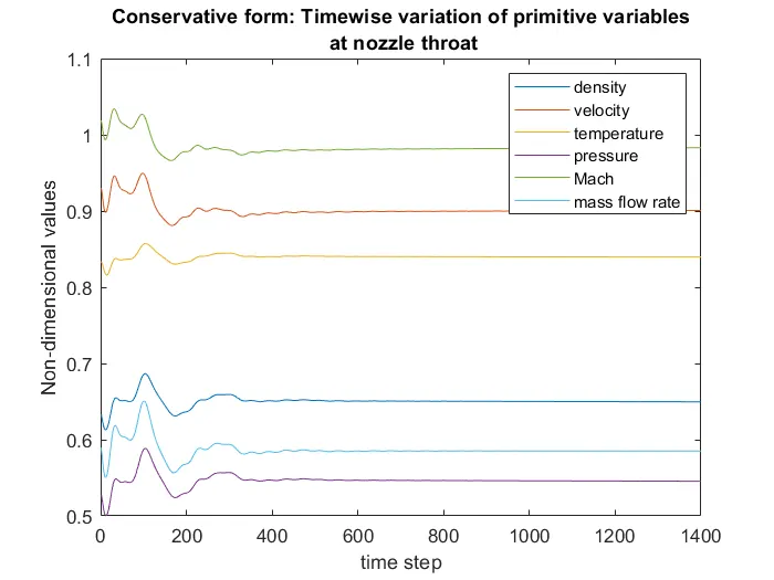
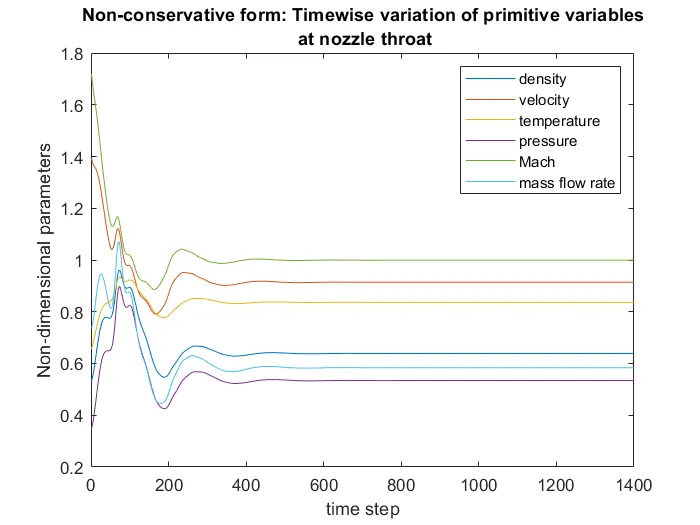
Before trying to analyze the steady state one-dimensional flow, we must justify the choice of the number of grid points are sufficient to fully reveal the flow physics. The values of the primitive variables at the nozzle throat are used for the verification of the conservative and the non-conservative forms. The number of grid points tested are 31 and 61 for both forms.
| Flow variables | rho | T | p | M |
| exact | 0.634 | 0.833 | 0.528 | 1 |
| Con 31 | 0.6497 | 0.8396 | 0.5455 | 0.983 |
| Con 61 | 0.6382 | 0.8351 | 0.533 | 0.9994 |
| Non-con 31 | 0.6386 | 0.8364 | 0.5341 | 0.9994 |
| Non-con 61 | 0.6375 | 0.8354 | 0.5326 | 0.9997 |
From this we conclude, that 31 grid points are sufficient for both implementations using the MacCormack's technique.
Simulation Code:
The conservative form's implementation using the MacCormack's technique is done by the conservative.m MATLAB function. The structure of the function is as follows:
- Conserved quantities U1, U2, U3 are calculated from the primitive variables, thermodynamic properties of the fluid and the area of the converging-diverging nozzle
- Fluxes F1, F2, F3 and source J2 are calculated from the conserved quantities U1, U2, U3 using their respective helper functions
- The outermost loop is for time marching because the PDE's are hyperbolic in time
- Inside the time loop, we first calculate the minimum time step from all the grid points using a Courant Number of 0.5
- The predictor step calculates the gradient using the forward difference scheme and the new values of U1, U2, and U3 are calculated using the Taylor approximation
- The boundary values are updated and the fluxes F1, F2 and F3 and source J2 are calculated using the updated values
- The corrector step calculates the gradient using the backward difference scheme with the updated values and then use these gradients to calculate the average gradient
- The U1, U2, and U3 values are updated using the average gradients and we calculate the primitive variables from the conserved quantities
- The primitive variables are plotted wrt time and length of nozzle to study the transient evolution of the flow and the steady state results
function [rho_f,V_f,T_f,p_f,M_f,mfr_f] = conservative(rho,A,x,T,gamma,V,mfr,...
                                                      C,dx,n,nt)
%% Conserved quantities and fluxes

U1 = rho.*A;
U2 = mfr;
U3 = rho.*(T./(gamma - 1) + gamma.*V.^(2)./2).*A;

F1 = F_1(U2);
F2 = F_2(U1,U2,U3,gamma);
F3 = F_3(U1,U2,U3,gamma);
J2 = J_2(T,rho,gamma);

U1_old = U1;
U2_old = U2;
U3_old = U3;


for t=1:nt

    % Calculation of timestep
    del_t = (C*dx)./(sqrt(T) + V);
    del_t = min(del_t);

    %Predictor step
    for i=2:n-1
            dU1_dt_1(i) = -(F1(i+1) - F1(i))/dx;
            dU2_dt_1(i) = -(F2(i+1) - F2(i))/dx + J2(i)*(A(i+1) - A(i))/dx;
            dU3_dt_1(i) = -(F3(i+1) - F3(i))/dx;
    end

    for i=2:n-1
            U1(i) = U1_old(i) + dU1_dt_1(i)*del_t;
            U2(i) = U2_old(i) + dU2_dt_1(i)*del_t;
            U3(i) = U3_old(i) + dU3_dt_1(i)*del_t;
    end

    %Boundary conditions
    rho = U1./A;
    V = U2./(rho.*A);
    T = (gamma - 1)*((U3./U1) - (gamma.*V.^(2))/2);

    U2(1) = 2*U2(2) - U2(3);
    v = U2(1)/(rho(1)*A(1));
    U3(1) = U1(1)*(1/(gamma-1) + (gamma/2)*v^(2));

    U1(end) = 2*U1(end-1) - U1(end-2);
    U2(end) = 2*U2(end-1) - U2(end-2);
    U3(end) = 2*U3(end-1) - U3(end-2);

    %Predictor updated fluxes
    F1 = F_1(U2);
    F2 = F_2(U1,U2,U3,gamma);
    F3 = F_3(U1,U2,U3,gamma);
    J2 = J_2(T,rho,gamma);

    % Corrector step
    for i=2:n-1
            dU1_dt_2(i) = -(F1(i) - F1(i-1))/dx;
            dU2_dt_2(i) = -(F2(i) - F2(i-1))/dx + J2(i)*(A(i) - A(i-1))/dx;
            dU3_dt_2(i) = -(F3(i) - F3(i-1))/dx;
    end

    for i=2:n-1
            dU1_dt_avg(i) = 0.5*(dU1_dt_1(i) + dU1_dt_2(i));
            dU2_dt_avg(i) = 0.5*(dU2_dt_1(i) + dU2_dt_2(i));
            dU3_dt_avg(i) = 0.5*(dU3_dt_1(i) + dU3_dt_2(i));
    end

    for i=2:n-1
            U1(i) = U1_old(i) + dU1_dt_avg(i)*del_t;
            U2(i) = U2_old(i) + dU2_dt_avg(i)*del_t;
            U3(i) = U3_old(i) + dU3_dt_avg(i)*del_t;
    end

    %Boundary conditions
    U2(1) = 2*U2(2) - U2(3);
    V(1) = U2(1)/(rho(1)*A(1));
    U3(1) = U1(1)*(1/(gamma-1) + (gamma/2)*V(1)^2);

    U1(end) = 2*U1(end-1) - U1(end-2);
    U2(end) = 2*U2(end-1) - U2(end-2);
    U3(end) = 2*U3(end-1) - U3(end-2);

    % Primitive variables
    rho = U1./A;
    V = U2./U1;
    T = (gamma - 1)*((U3./U1) - (gamma.*V.^(2))/2);
    p = rho.*T;
    M = V./sqrt(T);
    mfr = U2;

    %Updating fluxes
    F1 = F_1(U2);
    F2 = F_2(U1,U2,U3,gamma);
    F3 = F_3(U1,U2,U3,gamma);
    J2 = J_2(T,rho,gamma);

    %Updating old
    U1_old = U1;
    U2_old = U2;
    U3_old = U3;

    %primitive variables at throat
    rho_t(t) = rho(16);
    V_t(t) = V(16);
    T_t(t) = T(16);
    p_t(t) = p(16);
    M_t(t) = M(16);
    mfr_t(t) = mfr(16);

    %Plotting mass flow rate wrt position at certain times
    figure(1)
    if (t == 1 || t == 51 || t == 101 ...
       || t == 151 || t == 201 || t == 701 || t == 1400)
        if (t == 1400)
           plot(x,mfr,'*','DisplayName',sprintf('t=%d',t))
           hold on;
        else
            plot(x,mfr,'DisplayName',sprintf('t=%d',t))
            hold on;
        end
    end
    legend show
    ylim([0.4 1])

end

    rho_f = rho;
    V_f = V;
    T_f = T;
    p_f = p;
    M_f = M;
    mfr_f = mfr;

    %Plotting primitive variables at throat wrt time
    figure(2)
    plot(1:nt,rho_t,1:nt,V_t,1:nt,T_t,1:nt,p_t, ...
         1:nt,M_t,1:nt,mfr_t)
    legend('density','velocity','temperature','pressure',...
           'Mach','mass flow rate')

    %Plotting steady state primitive variables
    figure(3)
    plot(x,rho_f,x,V_f,x,T_f,x,p_f,x,M_f,x,mfr_f);
    legend('density','velocity','temperature','pressure','Mach','mass flow rate')

end
The helper functions for the calculations of the fluxes and sources are calculated are implemented for cleaner implementation of the algorithm
function [val] = F_1(U2)
val = U2;
end
function [val] = F_2(U1,U2,U3,gamma)
term1 = U2.^(2)./U1;
term2 = (gamma-1)/gamma;
term3 = U3 - gamma/2.*term1;
val = term1 + term2.*term3;
endfunction [val] = F_3(U1,U2,U3,gamma)
term1 = (gamma*U2.*U3)./U1;
term2 = gamma*(gamma-1)/2;
term3 = U2.^(3)./U1.^(2);
val = term1 - term2.*term3;
endThe non-conservative form using the MacCormack's Technique is implemented using the non_conservative.m MATLAB function. The structure of the code is as follows:
- No preprocessing because PDE's are in the primitive form
- The outermost loop is time loop for time marching
- We calculate the minimum time step by scanning all the grid points and using Courant number as 0.5
- The predictor step calculates the gradient using the forward difference and the primitive variables are updated using the Taylor's approximation
- Boundary values of the primitive variables are updated
- The corrector step calculates the gradient using the backward difference and the average gradient is calculated
- Calculate the updated values using the average gradients and apply the boundary conditions
- Plot the primitive variables wrt time and length to steady the transient evolution of the flow and the steady state results
function [rho_f,V_f,T_f,p_f,M_f,mfr_f] = non_conservative(rho,V,T,A,C,x,dx,...
                                                          gamma,n,nt)

rho_old = rho;
T_old = T;
V_old = V;

for t = 1:nt

    del_t = (C*dx)./(sqrt(T) + V);
    del_t = min(del_t);

    %Predictor step
    for i=2:n-1
        drho_dt_f(i) = drhodt_f(rho,V,A,dx,i);
        dV_dt_f(i) = dVdt_f(rho,V,T,gamma,dx,i);
        dT_dt_f(i) = dTdt_f(V,T,A,gamma,dx,i);
    end

    for i=2:n-1
            rho(i) = rho_old(i) + drho_dt_f(i)*del_t;
            V(i) = V_old(i) + dV_dt_f(i)*del_t;
            T(i) = T_old(i) + dT_dt_f(i)*del_t;
    end

    %Boundary Conditions
    rho(1) = 1;
    V(1) = 2*V(2) - V(3);
    T(1) = 1;

    V(end) = 2*V(end-1) - V(end-2);
    rho(end) = 2*rho(end-1) - rho(end-2);
    T(end) = 2*T(end-1) - T(end-2);

    %Corrector Step
    for i=2:n-1
        drho_dt_b(i) = drhodt_b(rho,V,A,dx,i);
        dV_dt_b(i) = dVdt_b(rho,V,T,gamma,dx,i);
        dT_dt_b(i) = dTdt_b(V,T,A,gamma,dx,i);
    end

    for i=2:n-1
        drho_dt_avg(i) = 0.5*(drho_dt_b(i) + drho_dt_f(i));
        dV_dt_avg(i) = 0.5*(dV_dt_b(i) + dV_dt_f(i));
        dT_dt_avg(i) = 0.5*(dT_dt_b(i) + dT_dt_f(i));
    end

    for i=2:n-1
            rho(i) = rho_old(i) + drho_dt_avg(i)*del_t;
            V(i) = V_old(i) + dV_dt_avg(i)*del_t;
            T(i) = T_old(i) + dT_dt_avg(i)*del_t;
    end

    %Boundary Conditions
    rho(1) = 1;
    V(1) = 2*V(2) - V(3);
    T(1) = 1;

    V(end) = 2*V(end-1) - V(end-2);
    rho(end) = 2*rho(end-1) - rho(end-2);
    T(end) = 2*T(end-1) - T(end-2);

    %Extra primitive variables
    p = rho.*T;
    M = V./sqrt(T);
    mfr = rho.*A.*V;

    %Update old variables
    rho_old = rho;
    T_old = T;
    V_old = V;

    %primitive variables at throat
    rho_t(t) = rho(16);
    V_t(t) = V(16);
    T_t(t) = T(16);
    p_t(t) = p(16);
    M_t(t) = M(16);
    mfr_t(t) = mfr(16);

    %Plotting mass flow rate wrt position at certain times
    figure(4)
    if (t == 1 || t == 51 || t == 101 ...
       || t == 151 || t == 201 || t == 701 || t == 1400)
        if (t == 1400)
           plot(x,mfr,'*','DisplayName',sprintf('t=%d',t))
           hold on;
        else
            plot(x,mfr,'DisplayName',sprintf('t=%d',t))
            hold on;
        end
    end
    legend show
    ylim([0.1 2])

end

    rho_f = rho;
    V_f = V;
    T_f = T;
    p_f = p;
    M_f = M;
    mfr_f = mfr;

    %Plotting primitive variables at throat wrt time
    figure(5)
    plot(1:nt,rho_t,1:nt,V_t,1:nt,T_t,1:nt,p_t, ...
         1:nt,M_t,1:nt,mfr_t)
    legend('density','velocity','temperature','pressure',...
           'Mach','mass flow rate')

    %Plotting steady state primitive variables
    figure(6)
    plot(x,rho_f,x,V_f,x,T_f,x,p_f,x,M_f,x,mfr_f);
    legend('density','velocity','temperature','pressure',...
           'Mach','mass flow rate')

end
The gradients of the primitive variables for the predictor and the corrector step are calculated using the helper functions for a cleaner implementation
function [val] = drhodt_b(rho,V,A,dx,i)

term1 = -rho(i)*((V(i) - V(i-1))/dx);
term2 = -rho(i)*V(i)*((log(A(i)) - log(A(i-1)))/dx);
term3 = -V(i)*((rho(i) - rho(i-1))/dx);

val = term1 + term2 + term3;

end
function [val] = drhodt_f(rho,V,A,dx,i)
term1 = -rho(i)*((V(i+1) - V(i))/dx);
term2 = -rho(i)*V(i)*((log(A(i+1)) - log(A(i)))/dx);
term3 = -V(i)*((rho(i+1) - rho(i))/dx);
val = term1 + term2 + term3;
endfunction [val] = dTdt_b(V,T,A,gamma,dx,i)
term1 = -V(i)*((T(i) - T(i-1))/dx);
term2 = (V(i) - V(i-1))/dx;
term3 = V(i)*(log(A(i)) - log(A(i-1)))/dx;
val = term1 - (gamma-1)*T(i)*(term2 + term3);
endfunction [val] = dTdt_f(V,T,A,gamma,dx,i)
term1 = -V(i)*((T(i+1) - T(i))/dx);
term2 = (V(i+1) - V(i))/dx;
term3 = V(i)*(log(A(i+1)) - log(A(i)))/dx;
val = term1 - (gamma-1)*T(i)*(term2 + term3);
endfunction [val] = dVdt_b(rho,V,T,gamma,dx,i)
term1 = -V(i)*((V(i) - V(i-1))/dx);
term2 = (T(i) - T(i-1))/dx;
term3 = (T(i)/rho(i))*((rho(i) - rho(i-1))/dx);
val = term1 - (1/gamma)*(term2 + term3);
endfunction [val] = dVdt_f(rho,V,T,gamma,dx,i)
term1 = -V(i)*((V(i+1) - V(i))/dx);
term2 = (T(i+1) - T(i))/dx;
term3 = (T(i)/rho(i))*((rho(i+1) - rho(i))/dx);
val = term1 - (1/gamma)*(term2 + term3);
endThe main.m MATLAB file calls both the solver code and compares the performance of the solver functions. The structure of the code is as follows:
- Setup the initial conditions of the primitive variables for conservative form, thermodynamic properties of the gas and discretization of the domain
- Calling the conservative MacCormack function
- Similarly for non-conservative MacCormack function
- Plotting the mass flow rate comparision between the two implementations
%%

clear
close all
clc

%% Setting up the conservative problem

n = 31;         % Number of space discretizations
nt = 1400;      % Number of time discretizations
m = 0.59*ones(1,n); % mass flow rate
gamma = 1.4;    % Ratio of heat capacities
C = 0.5;        % Courant Number
x = linspace(0,3,n); % non-dimensional space
dx = x(2) - x(1);

% non-dimensional area
A = 1 + 2.2.*(x - 1.5).^2;

% non-dimensional density
x1 = x(0.0<=x & x<=0.5);
x2 = x(0.5<=x & x<=1.5);
x3 = x(1.5<=x & x<=3.0);
rho(0.0<=x & x<=0.5) = 1.0;
rho(0.5<=x & x<=1.5) = 1.0 - 0.366.*(x2 - 0.5);
rho(1.5<=x & x<=3.0) = 0.634 - 0.3879.*(x3 - 1.5);

% non-dimensional temperature
T(0.0<=x & x<=0.5) = 1.0;
T(0.5<=x & x<=1.5) = 1.0 - 0.167.*(x2 - 0.5);
T(1.5<=x & x<=3.0) = 0.833 - 0.3507.*(x3 - 1.5);

%non-dimensional velocity
V = m./(rho.*A);

%non-dimensional pressure
p = rho.*T;

%% Calling conservative Maccormack

[rho_c,V_c,T_c,p_c,M_c,mfr_c] = conservative(rho,A,x,T,gamma,V,m,C,dx,n,nt);

%% Setting up the non-conservative Macormack

rho = 1.0 - 0.3146.*x;        % non-dimensional density
T = 1.0 - 0.2314.*x;          % non-dimensional temperature
V = (0.1 + 1.09.*x).*sqrt(T); %non-dimensional pressure

%% Calling non-conservative Maccormack
[rho_nc,V_nc,T_nc,p_nc,M_nc,mfr_nc] = non_conservative(rho,V,T,A,C,x,dx,...
                                                       gamma,n,nt);

%% Plotting comparision results
figure(7)
plot(x,mfr_nc,x,mfr_c);
legend('Non-conservative','Conservative')
Simulation Results:
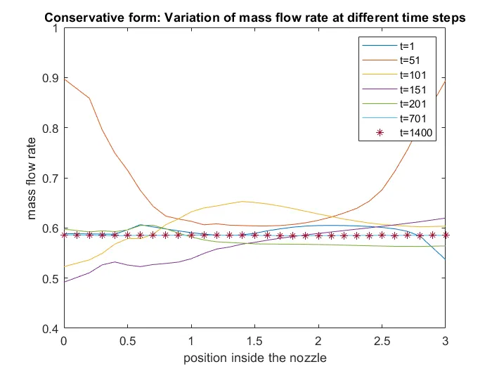
- Conservative form
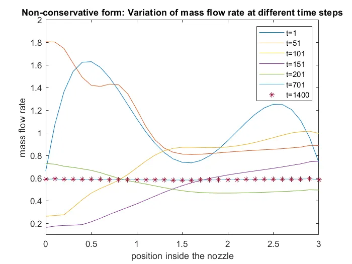
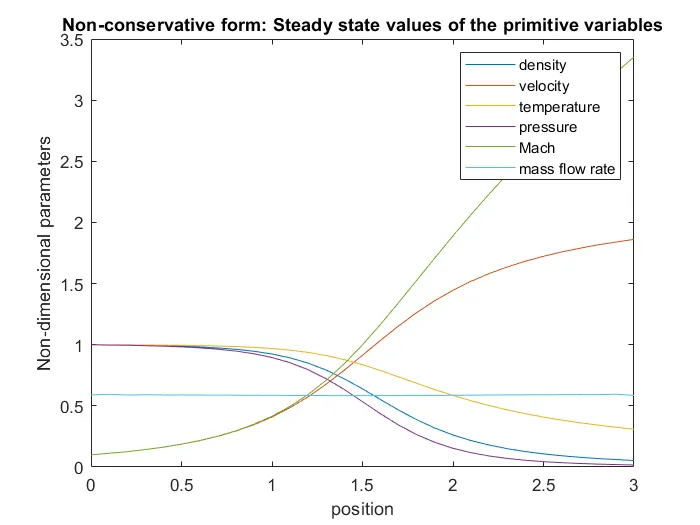
- Non Conservative
- Comparison of conservative and non-conservative
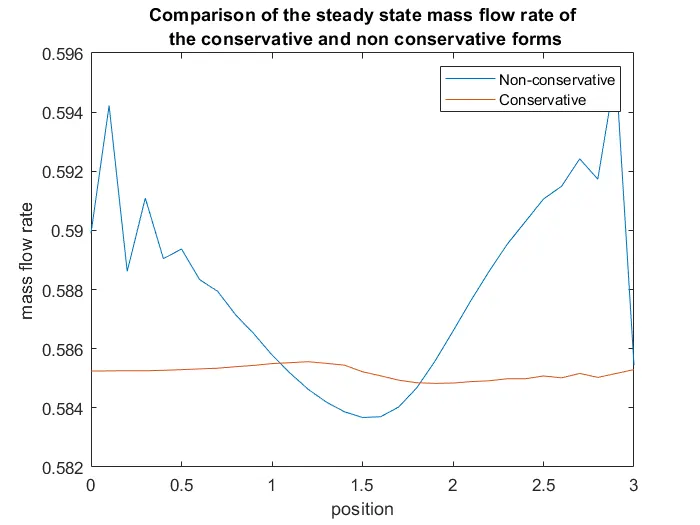
From the above algortithms and plots, we note the following observations:
- The conservative form implementation is more intense and can lead to numerical errors due to rounding off errors while the non-conservative form are easier to implement.
- The conservative and non-conservative methods reach to the steady state well before the 1400 time steps are completed.
- The convergence to steady state is faster in the conserved schemes compared to the non-conservative schemes.
- The values of the primitive variables at the throat are more accurate in the non-conservative scheme compared to the conservative scheme, even when finer meshes are used for the conservative schemes as observed in the grid independence.
- From the enlarged imaged of the mass flow rate at the final time step, we observe that non-conservative values are more oscillatory in nature while the conservative values have more consistent values throughout the domain
Conclusions:
Both formulations have their own advantages and disadvantages, but both of them provide a satisfactory steady state results for the current problem.
The real advantage of using the conservative formulation is observed while shocks are present, since the fluxes are conserved but the primitive variables themselves are discontinuous.