Week 10: Modeling and Simulation of flow around an Ahmed Body

Aim:

To model and simulate the flow around Ahmed body using a coarse mesh in Converge CFD and post-process the simulation results using Paraview.

Objectives:

1. Provide a brief introduction to the theory of flow over Ahmed body and calculations for Reynolds Number and wind tunnel dimensions
2. Generate the STL file for the Ahmed body using a standard CAD package
3. Generate mesh and setup simulation case for the Ahmed body using CONVERGE Studio
4. Post-process the simulation results by comparing the Drag and Lift coefficient from CONVERGE and Paraview
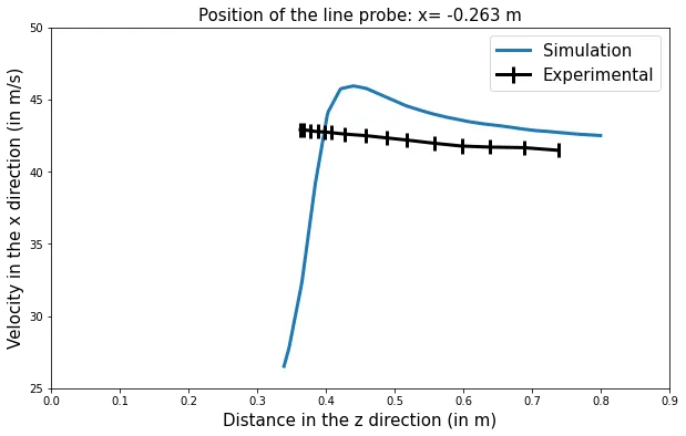
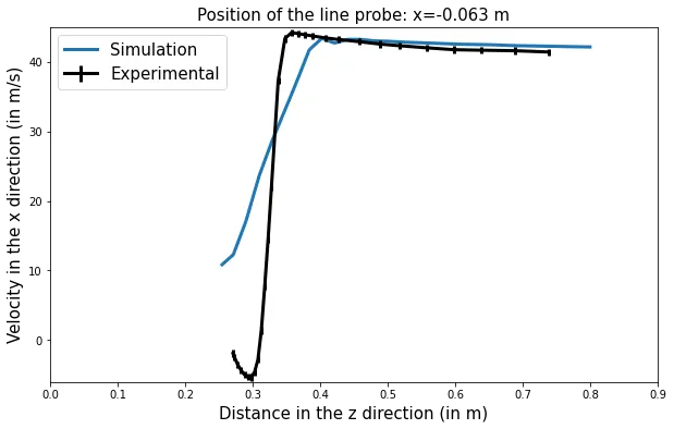
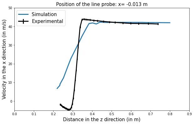
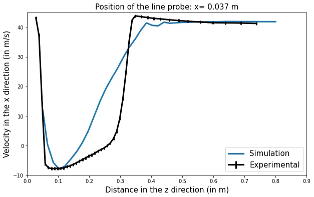
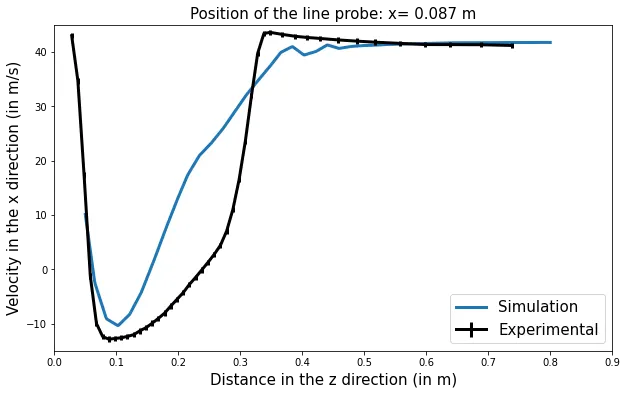
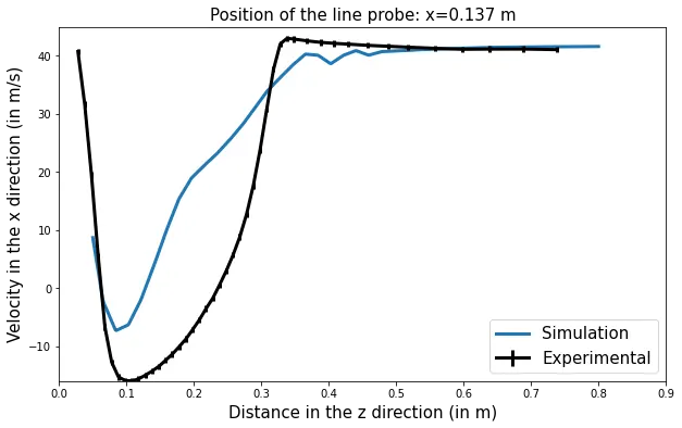
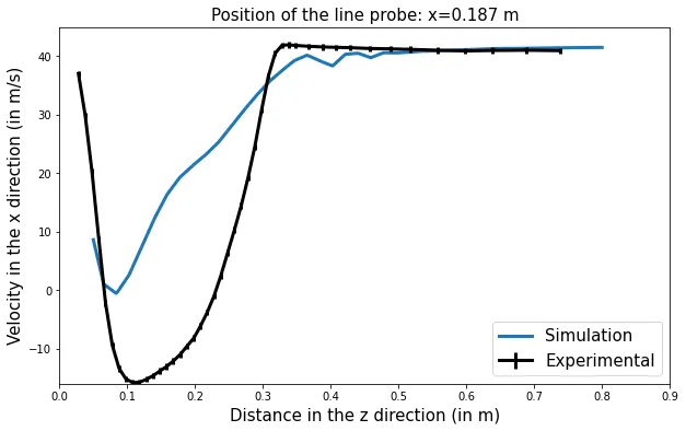
5. Compare the experimental data of velocity at different line probes with the simulation results
6. Summarise the insights gained from the project

Theory:

Although the Ahmed body seems simplistic in design, it capture all the essential geometrical features of a generic car. Because of this, the airflow around the Ahmed body mimics all the essential flow features around an automobile and these features were defined and characterized in the experimental work of Ahmed.

The main objective of this geometry is to validate the new numerical model of turbulence in the automobile industry. Once the model is properly validated by comparing experimental results, it is further employed to quantify the performance of the new models of the car.

Calculations:

The Reynolds number is described as the ratio of the inertial forces to viscous forces. Mathematically, it is represented by the following formula,

`Re = {u times L}/nu`

For the current simulation,

`u =`Characteristic velocity of the Air `= 40\ m//s`,

`L =` Characteristic Length of the domain = Height of the Ahmed body `= 0.288\ m` and

`nu =` Kinematic Viscosity of the air `= 15 times 10^-6\ m^2 // s`

Substituting these values, we get the following equation

`Re = {40 times 0.288}/{15 times 10^-6)`

`Re = 768,000`

---------------------------------------------------------------------------------------------------------------------------

For the simulation, we require a boundary layer of 30 mm thickness at 400 mm in front of the Ahmed body. For satisfying this constraint, we use the boundary layer thickness formula for flow over flat plate. This dimension will help us in determining the upstream length of the wind tunnel. Mathematically, the formula for boundary layer thickness for the flat plate can be,

`delta = {0.382 times x}/{Re^{1/5}}`

For the current simulation,

`delta =` Thickness of the boundary layer `= 0.03\ m`,

`Re =` Reynolds Number `= 768,000` and

`x =` Distance from the start of the flate plate

Substituting the known values in the equation and rearranging the terms we get the following equation,

`x = {delta times Re^{1/5} }/0.382`

`x = {0.03 times 768000^{1/5}}/0.382`

`x = 1.1806\ m`

---------------------------------------------------------------------------------------------------------------------------

In the streamwise direction of the flow in the wind tunnel we consider the following dimensions. First, 2 m of slip region, (1.18 + 0.4) m for generating 30 mm thicknes of boundary layer at a position of 400 mm ahead of the Ahmed body, 1.044 m which is the length of the Ahmed body and 6.264 m which if 6x length of the Ahmed body for accurately capturing flow physics in the down stream region.

Therefore, X = 2 + 1.18 + 0.4 + 1.044 + 6.264 = 10.888 m.

The y and z direction lengths are chosen in such a manner that their values are atleast bigger than the length of the Ahmed body and also accomodates a modest embedding region for finer resolution. This is done so that we do not violate the restriction on the maximum number of cells available with the Converge license.

Therefore, Y = 1.8 m and Z = 1.389 m.

Geometry:

The Ahmed body and the virtual wind tunnel is created using Onshape which is based on the above defined dimensions. The final geometry which is generated as a boolean operation between the Virtual wind tunnel and Ahmed body. The Geometry is represented as follows:

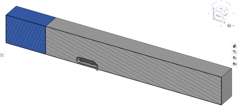
The geometry is then exported as STL File and imported into the CONVERGE Studio and the boundaries are flagged with appropriate names.

STL file in Converge CFD:

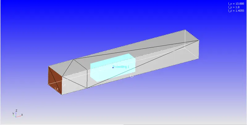
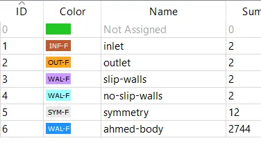
Case Setup:

The case setup for the current study is carried out using the CONVERGE Studio Case Setup GUI. The following settings have been chosen for the simulation in the respective subtree

• Application subtree:
  • Due to the relatively simple nature of the model, the Time based application was selected.

• Materials subtree:
  • Predefined mixture of standard air with gas simulation default settings was used.
  • The global transport parameters were set to default values.
  • The standard air consists of oxygen and nitrogen species which are assumed to be non-reacting mixtures.

• Simulation parameters subtree:
  • Fully compressible transient simulation with full hydrodynamic capacity is used for the simulation.
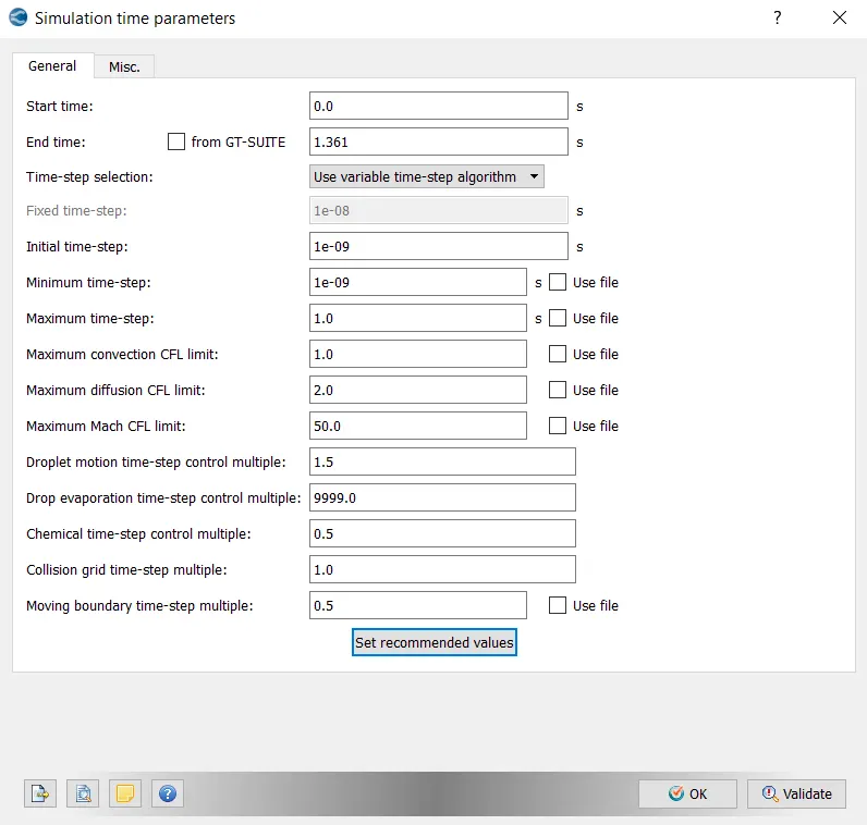
  • Using the inlet velocity of 40 m/s (for the Re = 768000) and the streamwise length of the domain of 10.888 m, we can calculated the flow through time as 0.2722. For achieving fully developed conditions, we decide the end time of the simulation as 1.361 seconds (5x flow through time).
  • The initial time step is set to 1e-9 which is also the minimum time step for the simulation. The maximum time step is set to 1 second. The CFL criteria for the convection is set to 1 and for diffusion is set as 2. The variable time-step algorithm is used for the time stepping in the problem.
  • A standard density based PISO algorithm was chosen as the Navier-Stokes equation solver with default settings

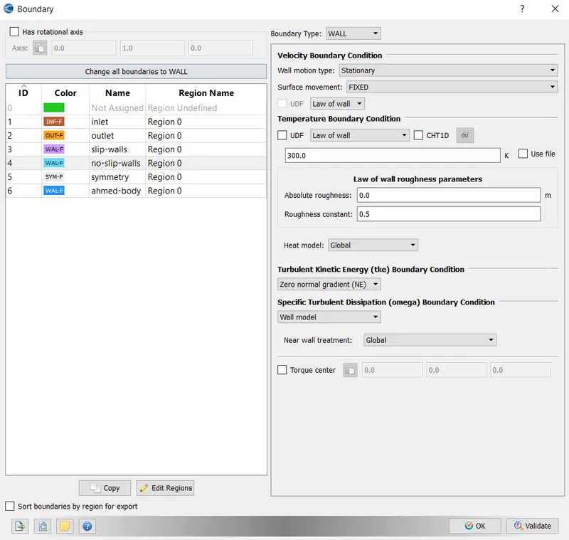
• Boundary Conditions subtree:
  • Inlet: Pressure = Zero Normal Gradient , Velocity = 40 m/s in the x-direction, Temperature = Fixed value of 300K, Species = Standard Air, Turbulent kinetic energy and turbulent frequency = default values
  • Outlet: Pressure = Static pressure of 101325 Pa (1 bar), Velocity = Zero Normal Gradient, Temperature = Backflow value of 300K, Species = Backflow value of Standard Air, Turbulent kinetic energy and turbulent frequency = default values
  • Ahmed body Wall: Pressure = zero normal gradient, Velocity = Law of the Wall (stationary), Temperature = Law of the wall with wall temperature as 300K, Turbulent kinetic energy = zero normal gradient and turbulent frequency= Wall model
  • Top and Side Walls: Symmetry.
  • Slip Bottom Wall: Pressure = zero normal gradient, Velocity= Slip, Temperature = zero normal gradient, Turbulent kinetic energy = zero normal gradient and turbulent frequency= zero normal gradient
  • No Slip Bottom Wall: Pressure = zero normal gradient, Velocity = Law of the Wall (stationary), Temperature = Law of the wall with wall temperature as 300K, Turbulent kinetic energy = zero normal gradient and turbulent frequency= Wall model

• Initial Conditions subtree:
  • Fluid domain is initialized by filling it standard Air with velocity equal to inlet velocity, temperature of 300K and pressure set at 101325 Pa.

• Physical Models subtree:
  
  • For the current simulation, k-`omega` SST turbulence models with automatic wall functions is used for the calculation of lift and drag forces.

• Grid Control subtree:
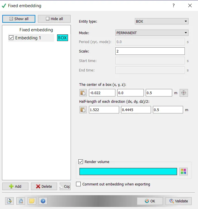
  • The base grid settings for cell dimension is set to 0.075 m in all directions.
  • A fixed embedding is provided in a box around the Ahmed body for finer resolution of the flow physics in the front and rear of the Ahmed body.

• Output subtree:
  • To calculate the forces in the principal directions on the Ahmed body, we switch on the wall output to boundaries only.

Simulation Results:

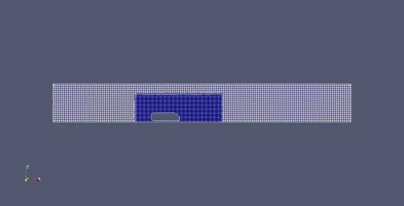
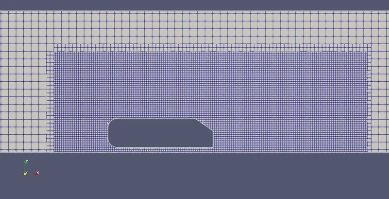
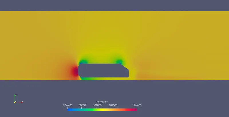
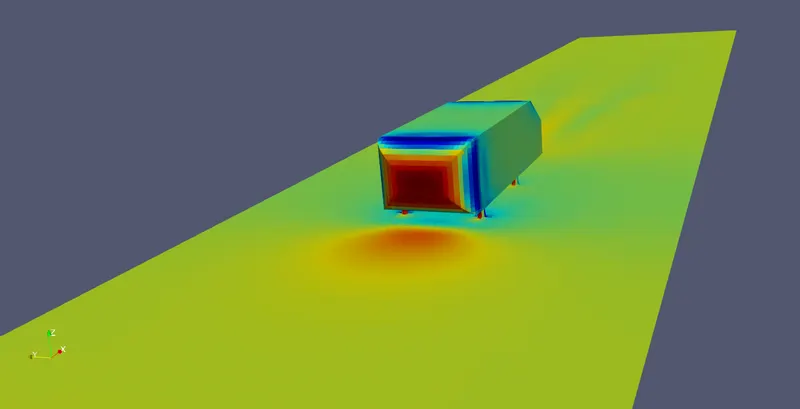
The post-processing of the simulation is carried out using the Paraview. The results are displayed in form of the mesh used for the simulation, velocity and pressure contours on a cutplane at the center of the computational domain, velocity and pressure contours on the Ahmed body which aids us identifying the locations where more mesh resolution is required, animations of the velocity and pressure contours, calculation of lift and drag using Converge and Paraview and comparision of the experimental data with the coarse mesh results.

Mesh:

Mesh closeup:

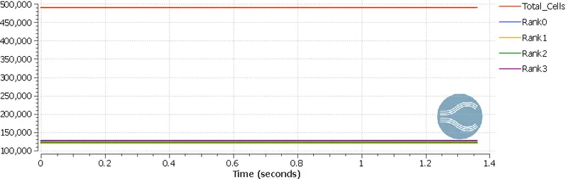
Number of Cells:

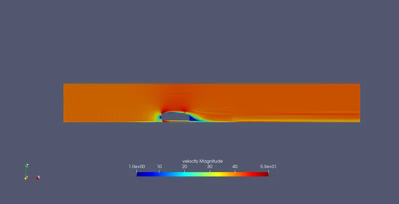
Velocity contour of the cut-plane:

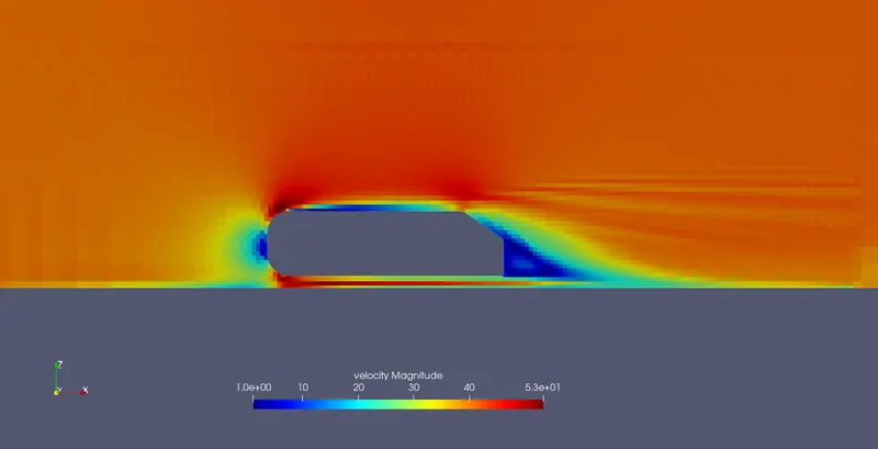
Velocity contour of the cut-plane closeup:

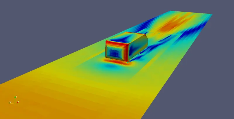
Velocity contour of the Ahmed Body frontside:

Velocity contour of the Ahmed Body backside:

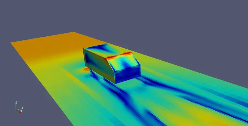
Pressure contour of the cut-plane:

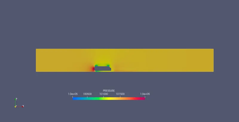
Pressure contour of the cut-plane closeup:

Pressure contour of the Ahmed Body frontside:

Pressure contour of the Ahmed Body backside:

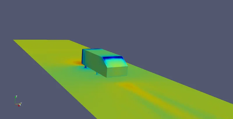
Velocity Animation: Animation Link

Pressure Animation: Animation Link

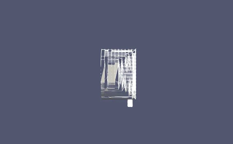
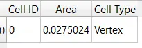
Frontal Area Calculation using Paraview:

Drag Force using Paraview:

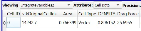
Lift Force using Paraview:

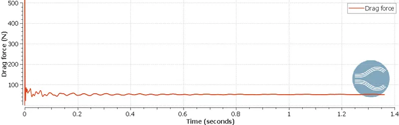
Drag force from wall averaged output from Converge CFD:

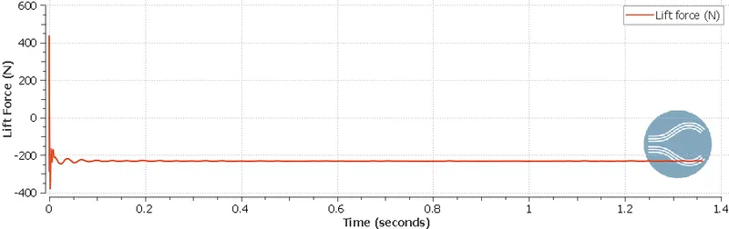
Lift Force from wall averaged output from Converge CFD:

Calculation of lift and Drag coefficients:

From literature, we know that lift and Drag coefficients are defined using the following formulaes

`C_D = F_D/{0.5 times rho times A times V^2}` and `C_L = F_L/{0.5 times rho times A times V^2}`

For this simulation,

`rho =` Density of the air `= 1.1761\ kg // m^3`,

`A =` Frontal Area `= 0.0275\ m^2`

`V =` Inflow velocity `= 40\ m//s`

`{rho times A times V^2}/2 = 25.8742`

---------------------------------------------------------------------------------------------------------------------------

Software	Drag Force	Drag Coefficient	Lift Force	Lift Coefficient
Paraview	25.6955	0.9931	-116.078	-4.4862
Converge Studio	51.350	1.985	-231.690	-8.9440

---------------------------------------------------------------------------------------------------------------------------

Comparision of experimental ans simulation results:

Probe 1:

Probe 2: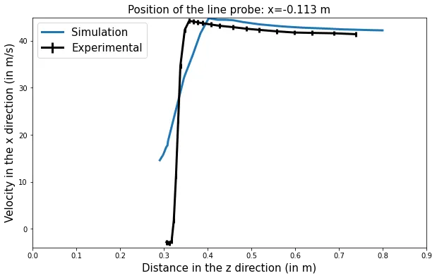

Probe 3:

Probe 4:

Probe 5:

Probe 6:

Probe 7:

Probe 8:

Conclusions:

From the above contours and plots we can make the following observations and conclusions:

• A successful simulation of the Ahmed body with coarse mesh is carried out and its results have been post-processed.
• The drag and lift forces and also the coefficients are 2x the value from the wall averaged data compared to the one from the Paraview since the Paraview related values are calculated only for the half region of the geometry.
• The lift force has a negative value, which means that force in pushing the Ahmed body towards the bottom wall.
• The velocity probes on the surface of Ahmed body have large error as the cell size for the current simulation is too large to appropriately capture the flow physics of the flow separation of the boundary layer.
• The velocity probes in the downstream direction show that the simulation follows the trends of the experimental observations but the wake region predicted by the simulation is smaller and weaker than what is actually observed in practice.