Week 3 - External flow simulation over an Ahmed body.

Aim:

To carry out grid independence study for flow over Ahmed body using ANSYS Fluent.

Objectives:

1. Provide brief historical and theoretical introduction on the flow physics over the Ahmed body (its importance in the automobiule industrial reseach).
2. Carry out grid dependence study for the external flow simulation using advanced meshing strategies.
3. Post process the simulation results and report the optimal mesh for the current simulation

Introduction:

The conception of Ahmed body was done by S.R Ahmed. This simplified model of a passenger automobile was used because simulating real geometries of the car is an extremely difficult and tedious process. The fuel consumption in automobiles depend on several parameters and a balance of those variables are required to make the vehicle fuel efficient. One of these parameters is the drag force acting on the car's body. The main purpose of Ahmed body model is to obtain a rough estimate on the drag force because of the car's geometry. This estmation helps us to determine whether the simulated geometry is fuel efficient.

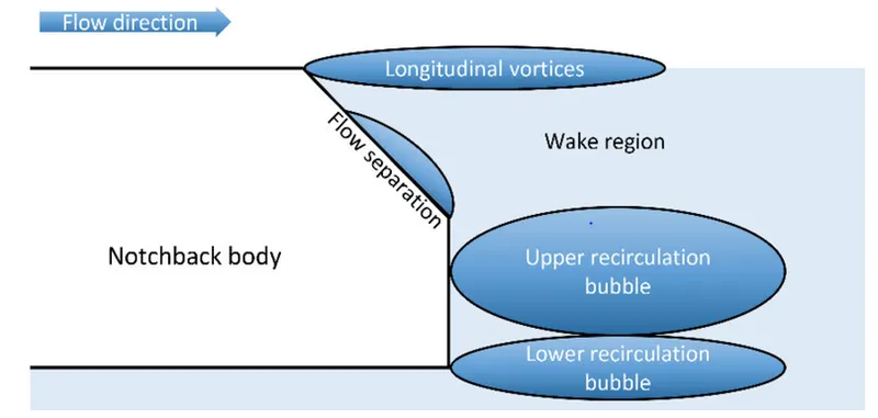
The drag force in Ahmed body is observed due to pressure drag generated because of the body's geometry. This happens due to formation of the low pressure turbulent zone in the terminal region of the geometry which is known as the wake region. The wake region are formed due to flow separation occuring in the rear part of the geometry. This separation also gives rise to several vorticial structures which are shown in the following figure

Separation at the boundaries occurs because of two reasons: discontinuity in the slope of the boundary or adverse pressure gradients. The flow inside the boundary layer slows down because of the viscous forces and if the pressure gradient is adverse then a recirculation region is created. The argument is presented visually using the following image

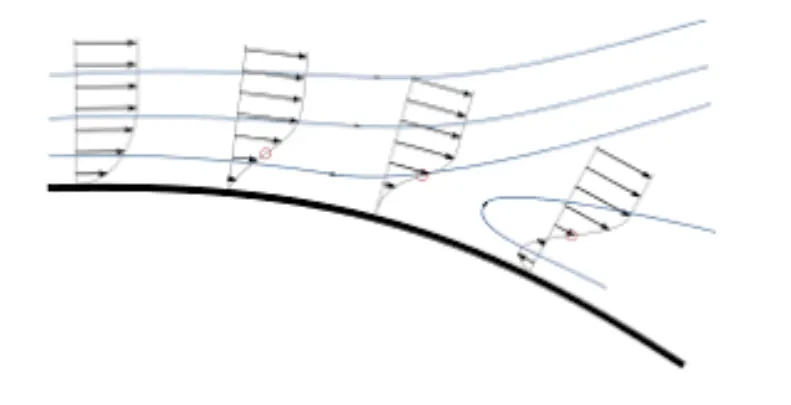
The fluid upstream the recirculation region gets detached because of the recirculating flow and this leads to the formation of the low pressure region in the rear part of the geometry. To prevent such flow separation it is advisable to make geometry more streamlined, avoiding sharp corners and utilizing the flow modifications technologies which energizes the boundary layer.

Geometry:

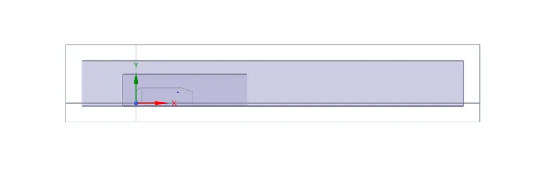
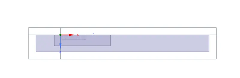
For the current study, Ahmed body has the following dimensions: the length along the flow is around 1.044 m, the height is 0.288 meters and the width is 0.389 meters. It rests on four pillars of 50 millimeters of height. The rear surface has a slant of 35 degrees with the x-axis direction. Since the body is symmetrical along the z-axis, we only take half of the geomery in consideration for the simulation. This strategy allows us to reduce the size of the computational domain thus decreasing the simulation time and make more refined mesh for achieving accurate results.

For simulating the external flow around the Ahmed body we also require to make a bounding box around it. This is done using the build-in tool of SpaceClaim known as the Enclosure. For the baseline mesh, we only use the single bounding box while for the refined meshs we utilize two bounding boxes to generate a refined mesh near the Ahmed body.

The following image summarizes all the geometrical information of the simulated Ahmed body. Here we only depict the refined mesh case for the sake of brevity.

Meshing:

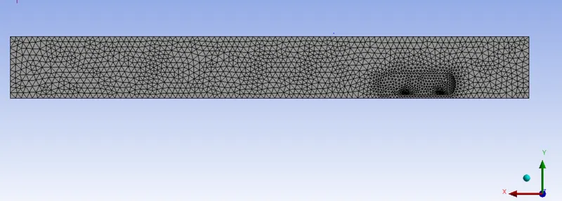
For the baseline mesh, we use a tetrahedral mesh with element size of 75 millimeters. For better resolution of the mesh on boundaries of the car walls, we use face sizing of 37.5 millimeters on the car-walls. The baseline mesh is shown in the following image:

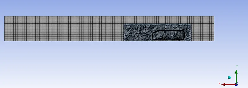
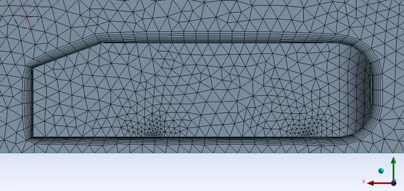
For the refined meshes, we use a multizone mesh method, for the mesh in the first bounding box is a quadrilaterial mesh with the element size 75 millimeters. The inner bounding box for refining the mesh around the Ahmed body, element size varies form 25 millimeters to 20 millimeters for different meshes and are called as the Refined 1, Refined 2 and Refined 3 from this point onwards. For properly resolving the flow close to the walls of the Ahmed body, we add 10 inflation layers with total thickeness of 37.2 millimeters, with the first layer cell thickness of 1 millimeters for y+ value of 100.

To visualize the above settings for the refined meshes, we depict Refined 1 Mesh and a close up view, which area as follows

The faces of the computational domain are assigned with appropriate labels which helps us to assign them proper boundary conditions in the Fluent GUI.

Case Setup:

The case setup for the baseline and the refined meshes are almost identical except the turbulence model. The settings for the case setup are as follows

• General
  • Since we are only interested in the time-averaged flow properties, a pressure-based steady state solver is chosen for the study.
  • The velocity formulation is chosen as absolute.
• Models
  • For the baseline mesh, we use the standard k-`epsi` model with standard wall functions for the near wall treatment. This is not recommended as we know that flow separation occurs but we can get a rough estimate for the flow parameters quickly using this model.
  • Since y+ value of 100 is used for determining the first cell thickness of the inflation layer, we observe that the viscous sublayer is not resolved and the first cell is present the log law region. Thus we use realizable k-`epsi` with non-equilibrium wall functions for near wall treatment to take into account the effects of adverse pressure gradientson the velocity profiles.
• Materials
  • Standard air from the Fluent database is set as the working fluid.
• Boundary Conditions
  • Inlet: A velocity of 25 m/s is set normal to the boundary.
  • Outlet: A pressure outlet with 0 gauge pressure is set at the outlet boundary.
  • Car walls: All the faces of the Ahmed body are assigned with stationary, no-slip walls
  • Symmetry: All the external facing walls of the bigger and smaller boundary box are assigned with the symmetry boundary conditions.
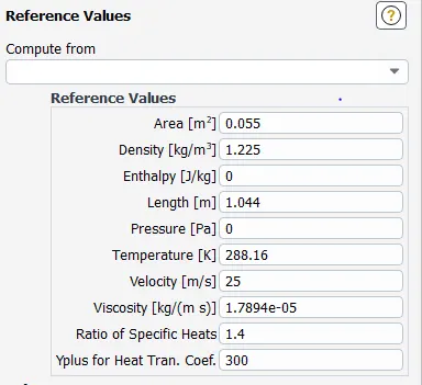
• Reference values for the current study for all the cases are set as follows

• Report Definitions
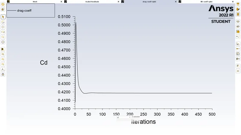
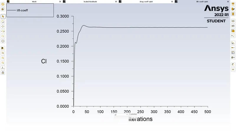
  • We setup a monitor for the drag and lift force coefficients for the car-walls.
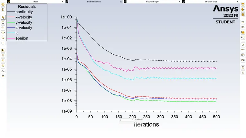
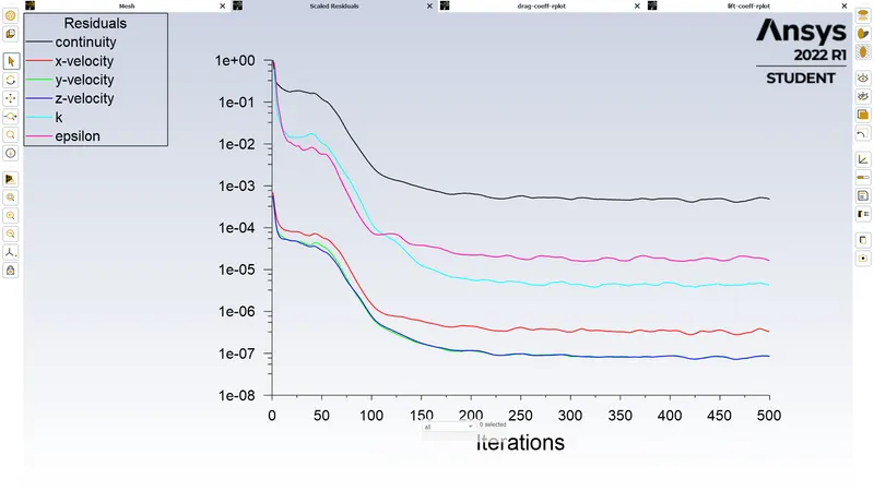
  • This will help us to observe the evolution of these parameters with the iterations and can help us to understand whether the flow has reached "convergence", as residuals do not provide much information as they show an oscillatory behavior after some number of iterations.
• Initialization
  
  • To provide a good intial guess for the velocity profile, we use the hybrid initialization for 20 iterations to reach the convergence tolerance of `10^{-6}`.
• Calculation activites
  • To observe the evolution of the velocity around the Ahmed body, we setup a cut plane animation of the velocity contours.
• Calculations
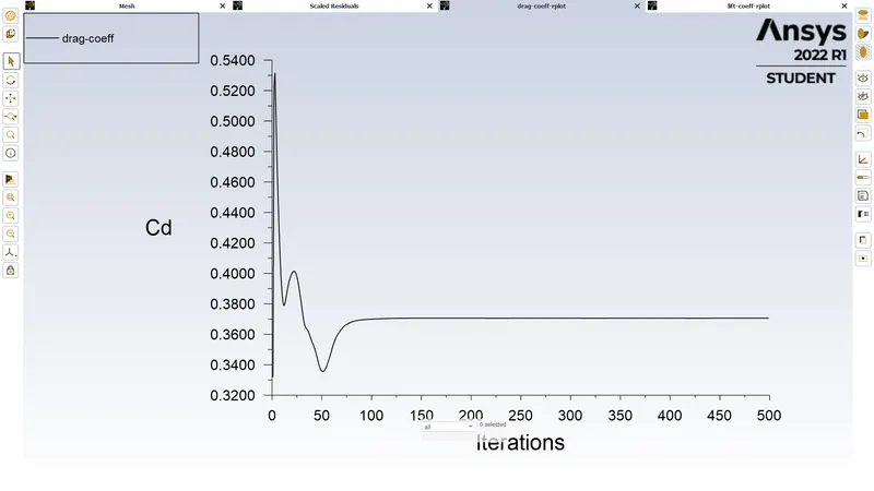
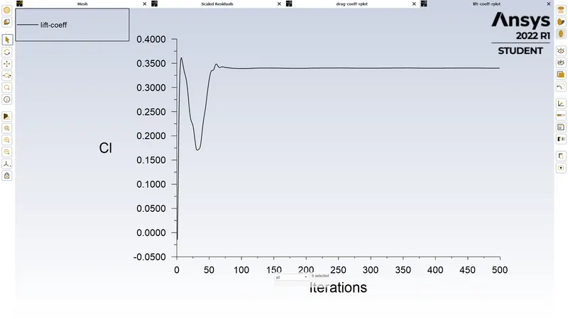
  • For all simulations for this study, we observe that they reach converged value for the drag and lift coefficients within 500 iterations.

Simulation results:

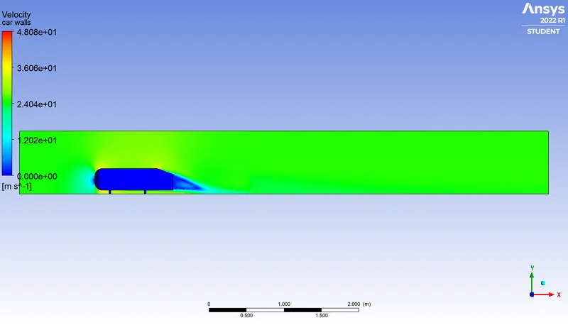
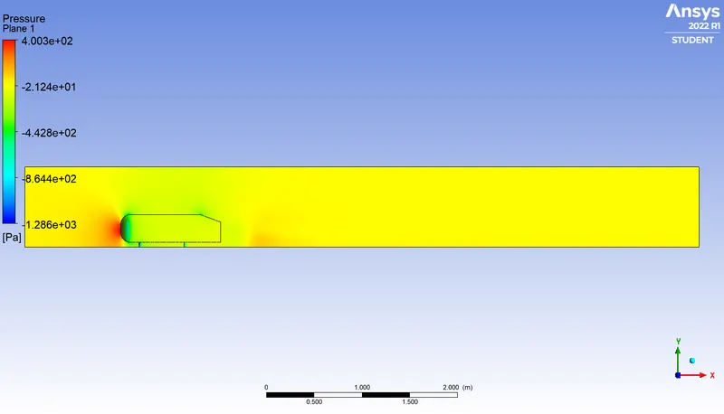
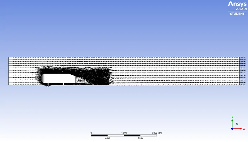
The simulation results for all the meshes are visualized below using contour and line plots. For this section, we carry out the grid dependence study based on the drag coefficient.

Baseline Mesh

• Residuals variation with number of iterations

• Drag Coefficient variation with number of iterations

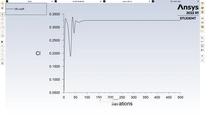
• Lift coefficient variation with number of iterations

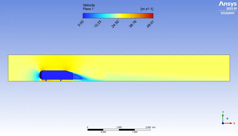
• Velocity contour

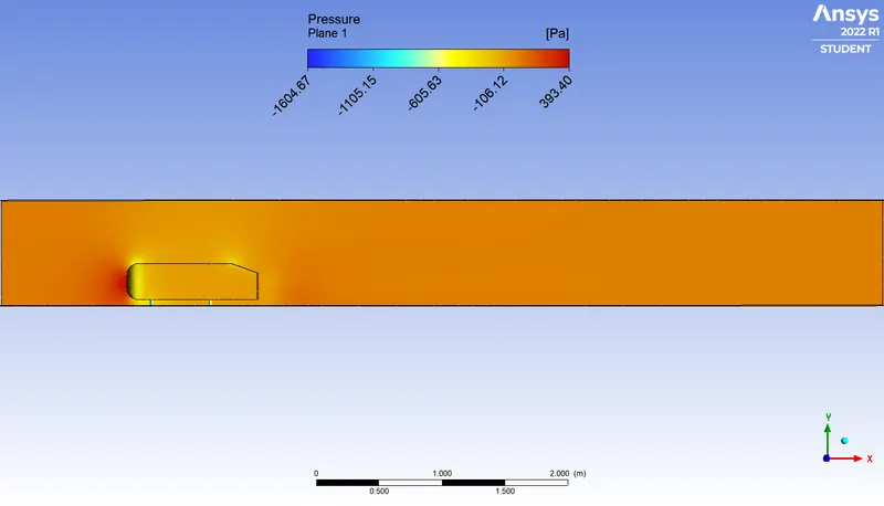
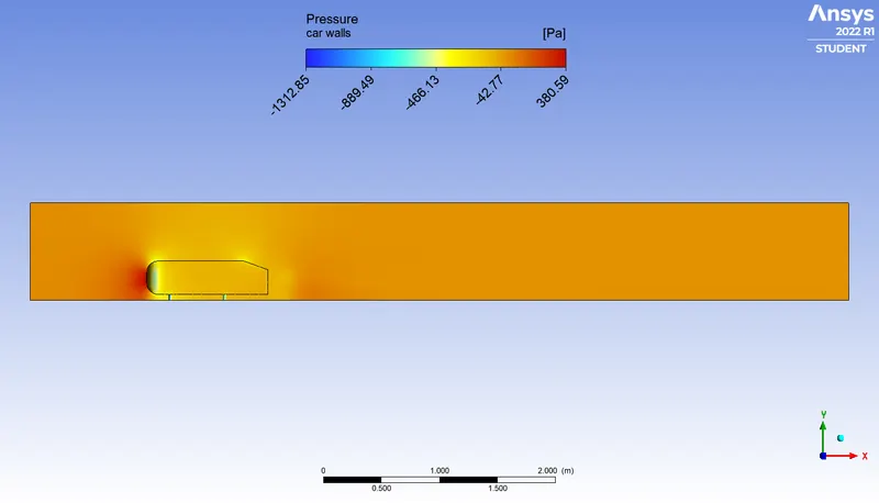
• Pressure contour

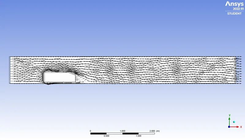
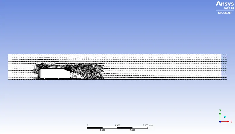
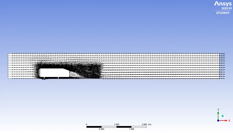
• Velocity vector plot

Refined Mesh 1

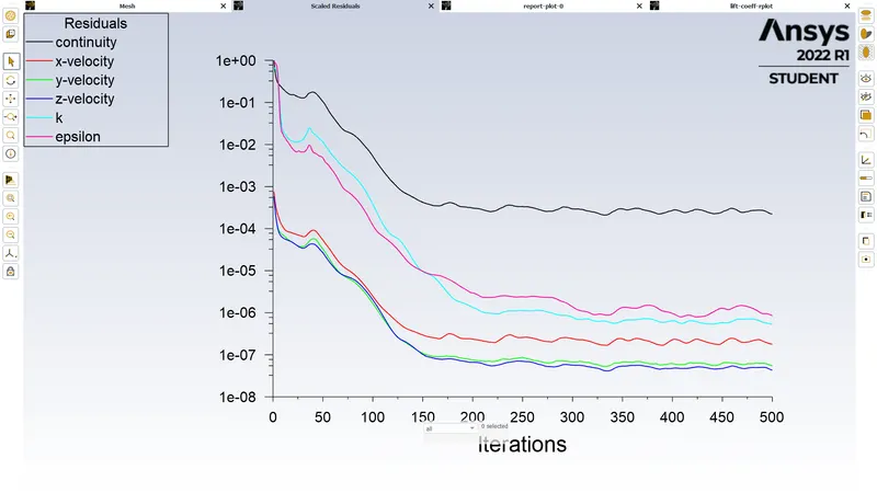
• Residuals variation with number of iterations

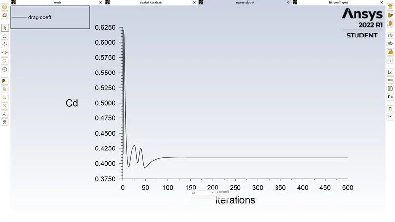
• Drag Coefficient variation with number of iterations

• Lift coefficient variation with number of iterations

• Velocity contour

• Pressure contour

• Velocity vector plot

Refined Mesh 2

• Residuals variation with number of iterations

• Drag Coefficient variation with number of iterations

• Lift coefficient variation with number of iterations

• Velocity contour

• Pressure contour

• Velocity vector plot

Refined Mesh 3

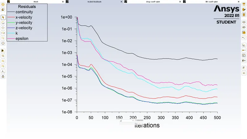
• Residuals variation with number of iterations

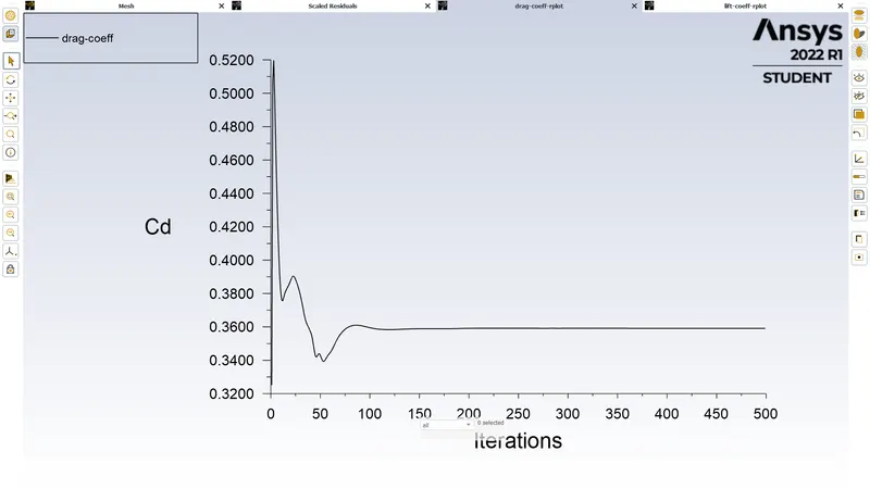
• Drag Coefficient variation with number of iterations

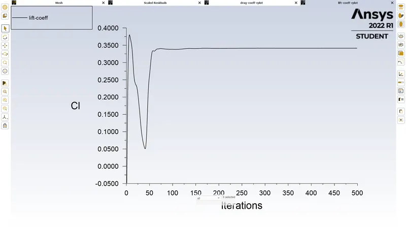
• Lift coefficient variation with number of iterations

• Velocity contour

• Pressure contour

• Velocity vector plot

From the above plots and contours we can make the following conclusions:

1. Results obtained for all the cases are converged by observing the oscillatory behavior of the residuals and the steady values of the lift and drag coefficients on the Ahmed body.
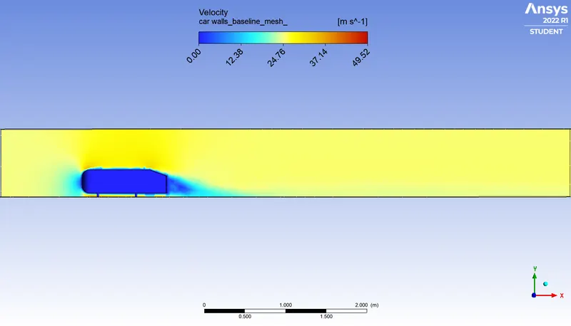
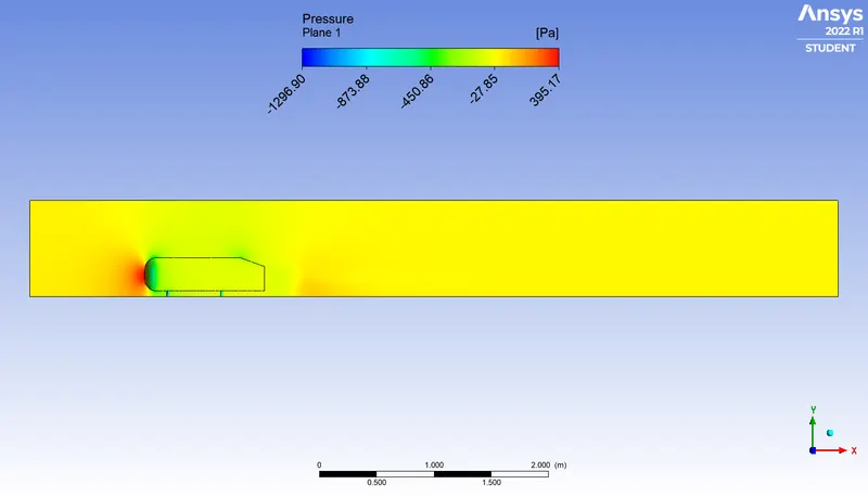
2. We can observe the wake region in the rear of the Ahmed body for all simulations but for the baseline case the wake velocity profile seems diffused.
3. The wake region is also identified using the velocity vector plots.
4. We observe that as the mesh resolution is increased the flow near the Ahmed body is resolved more accurately and the flow parameters such as drag and lift coefficient much closer to their theoritical counterpart.

To summarize the results of the mesh dependence study, we make a table and compare the drag coefficient and the number of cells present in the mesh

Mesh	Drag Coefficient	Number of cells
Baseline	0.42	115836
Refined 1	0.41	119860
Refined 2	0.37	282156
Refined 3	0.36	496441
Theoritical	~0.33	-

We observe that increasing the number of cells the drag coefficient becomes more close to the theoritical values. The relative increase in accuracy is much higher when mesh is refined from Baseline to Refined 2. After this, almost doubling the cell count from Refined 2 to Refined 3, the drag coefficient improves by limited fashion. Hence, for further analysis, Refined 2 mesh can be chosen.