Week 2 - Flow over a Cylinder.
Aim:
Simulating the classical case of flow over a circular cylinder and observing the Karman vortex street phenomenon.
Objectives:
- Brief introduction to theory of flow over cylinder.
- Generate the 2D surface with the circular cylinder.
- Mesh the 2D surface by using best practices for meshing circular geometry.
- Setup and simulate steady and unsteady flow over the cylinder for Reynolds number 100.
- Post-process the simulation results for the above simulations by calculating Strohaul Number, coefficient of lift and coefficient of drag and verify the findings with literature.
- Setup and simulate flow over cylinder for various reynolds numbers (10-100000) in the laminar and turbulent domains.
- Post-process the simulation results for the above simulations by calculating coefficient of lift and drag and verify the findings with literature.
Introduction:
The flow over cylinder remains an interesting problem in the field of CFD till date due to complex flow physics observed for the relatively simplistic nature of the geomtery. The complexity arises from the flow seperation on the sirface of the cylinder due to the adverse pressure gradient generated while flowing around the cylinder. This flow separation results into the formation of the cylinder wakes which are shed from the walls in a perodic fashion, giving rise to the popular phenomenon known as Karman vortex-street. Generally, the flow separation in CFD occur due to the presence of sharp edges in the geometry but in this case the separation occurs due to upstream boundary layers and non-dimensional numbers like Reynolds Number etc. As a result, exhaustive investigations must be carried out for understnading the effects of the domain and boundary conditions used for the CFD analysis.
The evolution of the flow is very much dependent on the non-dimensional number known as the Reynolds Number. This non-dimensional parameter is defined as the ratio of the inertial forces to the viscous forces. The wakes which are shed form the walls of the cylinder are observed to have periodic motion and such dynamics might have a characterstic frequency at which resonance occurs. This phenomenon is very important design consideration while designing any structure as it can lead to unwated motions which might compromise the system. The frequency of the oscillation can be non-dimensionalized by using the characteristic length and velocity of the domain. This is called as the Strohaul Number.
These phenomenon is observed in nature and industry for very complicated geometries. The current model proves to be a perfect surrogate for understanding the complex flow physics for vortex shedding and can provide useful insights for efficient designing.
Geometry:
The nature of the geometry in the study is simplistic, hence we create the surface in the ANSYS Spaceclaim tool. An illustration of the geometry is as follows.
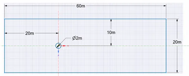
From the above image, we can observe that the diameter of the cylinder is 2m. The distance between the inlet and the center of the cylinder is 20m and the distance between the inlet and outlet of the domain is 60m. The horizontal boundaries of the domain are at distance of 10m from the center of the cylinder.
After sketching the geometry on the x-z plane, we generate the surface by pressing the "Pull" command present in Spaceclaim Toolbar.
Meshing:
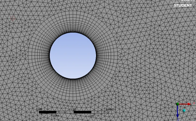
For the current simulation studies, we choose the base element as 0.19m which is ~1/10 of the characterisitic length and the cell generation method to all triangles method. To appropriately model the curvature of the cylinder, such that there are no sharp edges which can interfere with flow separation, we set the number of edges on the cylinder walls as 72. To accurately model the flow phyics near the walls of the cylinder, we add inflation layers. The first layer is `5 times 10^{-3}` m in height and growth rate of 1.2. To have some transition from the cells near the wall to the cells away form the walls, the number of the inflation layers is set to 20. The illustrations of the mesh and the close up to the walls of the cylinder are shown as follows:
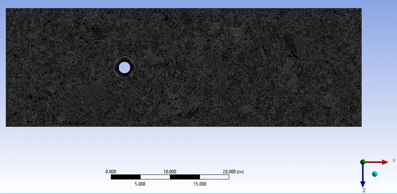
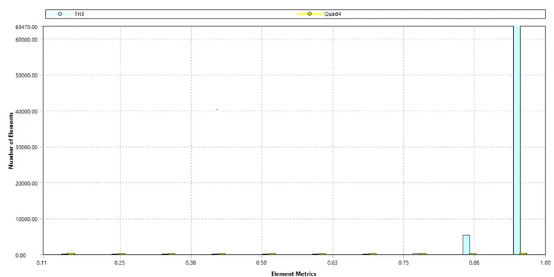
From the mesh statistics, we find that the total number of elements in the domain is 70240. To validate the mesh, we observe the following mesh metrics:
- Elements Quality:
- Skewness:
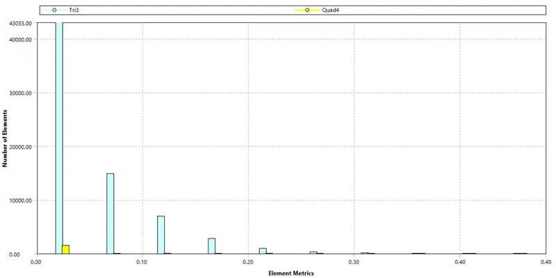
From the above mesh analysis, we can conclude that the almost all of the cells of the compuational domain have high quality and low skew number. We can conclude that mesh is appropriate for the simulations of the current study.
Case setup for steady and transient analysis:
The simulation cases for the current study are setup using ANSYS Fluent toolkit. The settings for both types of simulation modes are summarized as follows.
- General
- The solver is set to pressure-based and the velocity formulation is absolute.
- The time is set to steady or transient depending upon the nature of the simulation.
- Models
- The viscous model for the current simulation is set to laminar as we would like to resolve the separation of the boundary layers.
- For higher Reynolds number, it is appropriate to use K-`omega` SST model which is accurate for flows with separation near the walls.
- Materials
- For the study, we create a custom fluid and set it as the working fluid for the current simulations. The physical properties of the fluid are set as follows: Density = 1 kg/m3 and viscosity as 0.02 kg/ms.
- Boundary conditions
- Inlet: Velocity normal to the face depending on the Reynolds number (Re considered for the study are 10, 100, 1000, 10000, 100000).
- Outlet: Pressure outlet with gauge pressure value set to 0.
- Wall: The walls of the cylinder are stationary walls with no-slip conditons
- Symmetry: The symmetry boundaries are provided with symmetry boudnary conditions.
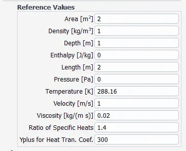
- Reference values
- The reference values are set according to the following figure
- Methods
- For the steady state simulation, the presure velocity coupling is performed using the SIMPLE Algorithm while for the transient simuation we use the Fractional step algorithm which provides results quickly with sufficient accuracy.
- Report Definitions
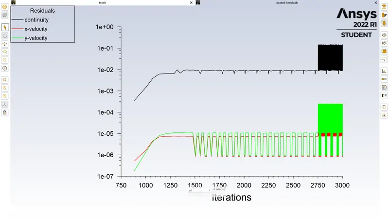
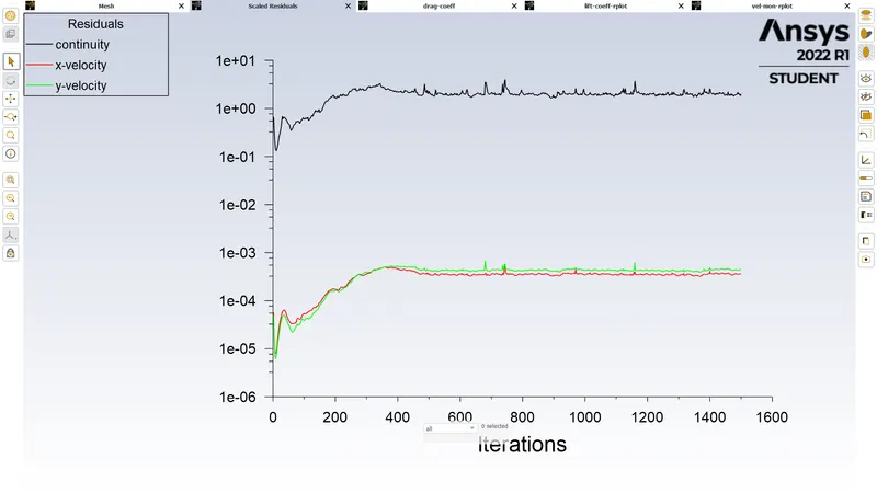
- Since the current simulation has oscillating flow nature, the residuals cannot provide accurate information of the convergence. Hence, we have created several monitors of velocity at a point near the outlet and lift and drag monitors for observing the flow oscillations and to decide whether the simulation has converged or not.
- Calculation activites
- After initializing the solution, we plot the contours of velocity to get an idea about the values used by the solver as the initial values for the calculations.
- Next, to observe how the flow field is evolving during the course of the simulation we setup the solution animations to update the velocity contours after a given amount of iterations
- Calculation
- We run the simulation for 300 seconds for the transient case and 1000 iterations for the steady case. These values are obtained by running extra iterations after running some intial amount iterations till a steady oscillating values for the velocity monitor and lift coefficient is obtained.
Steady state and Transient analysis for Re=100:
The current simulations are set up using the above steps. In this section, we will summarize the results obtained from the simulation and compare them with the values obtained in the literature.
Steady State simulation:
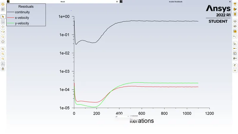
- Residual Plots vs number of iterations
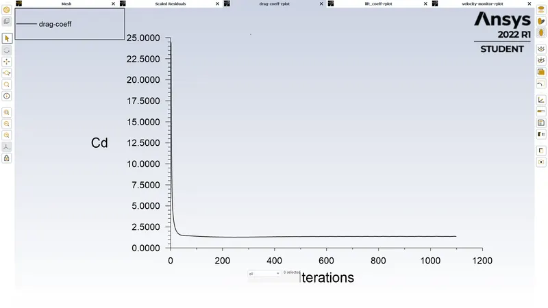
- Drag Coefficient vs number of iterations
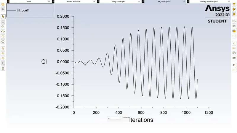
- Lift Coefficient vs number of iterations
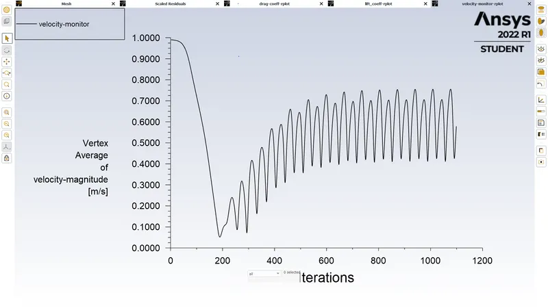
- Velocity magnitude at monitor point vs number of iterations
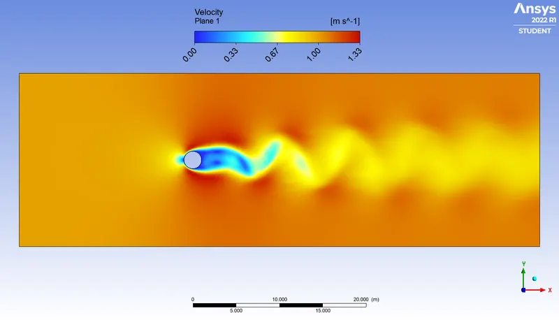
- Velocity Contour plot at the final iteration
Transient state simulation:
- Residual Plots vs number of iterations
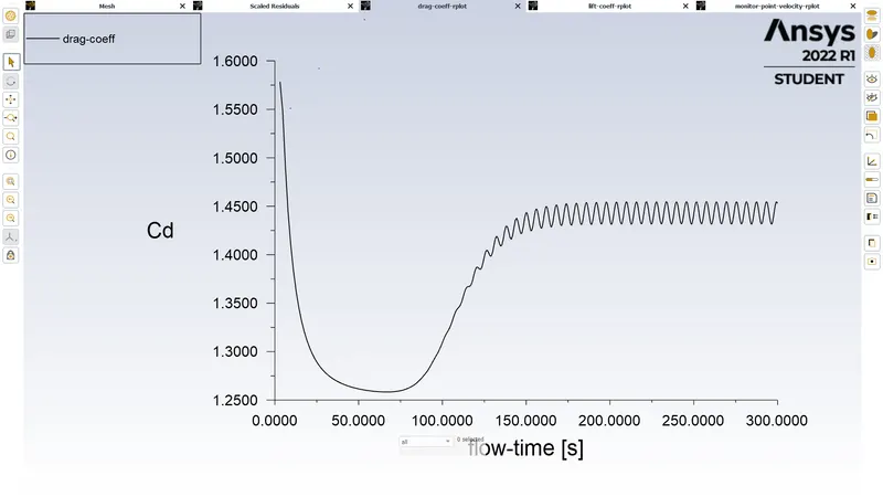
- Drag Coefficient vs number of iterations
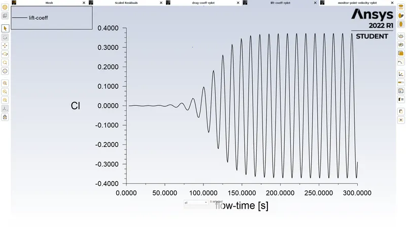
- Lift Coefficient vs number of iterations
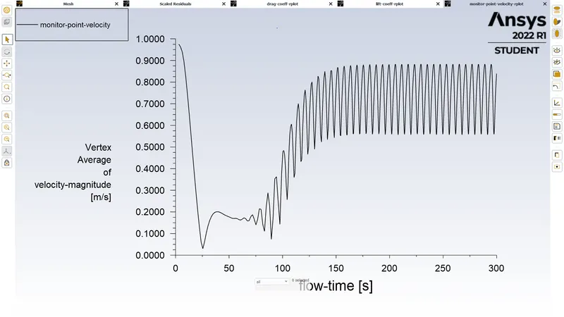
- Velocity magnitude at monitor point vs number of iterations
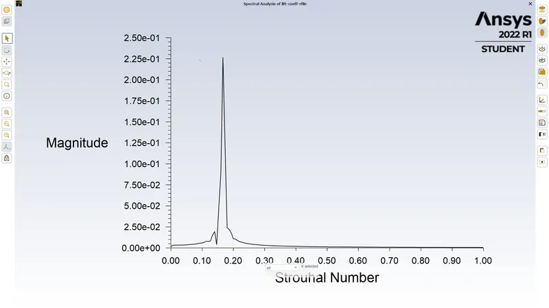
- Strohaul Number plot for the transient simulation
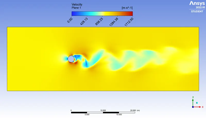
- Velocity Contour plot at the final time step
From the above figures, we can conclude the following statements:
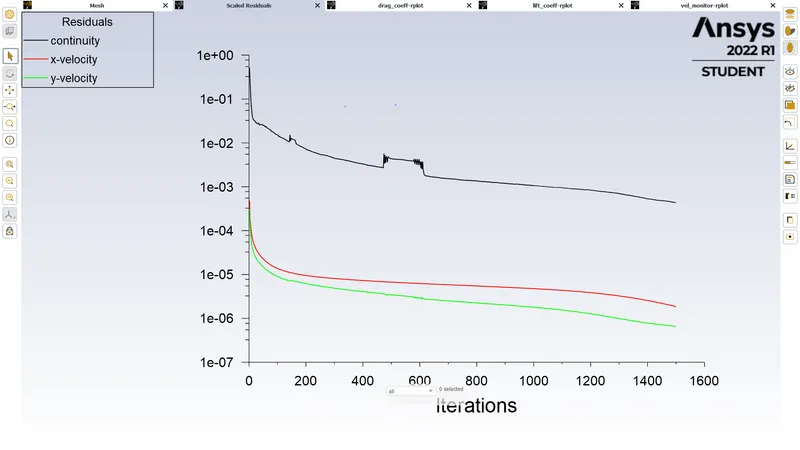
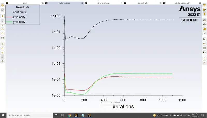
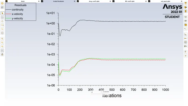
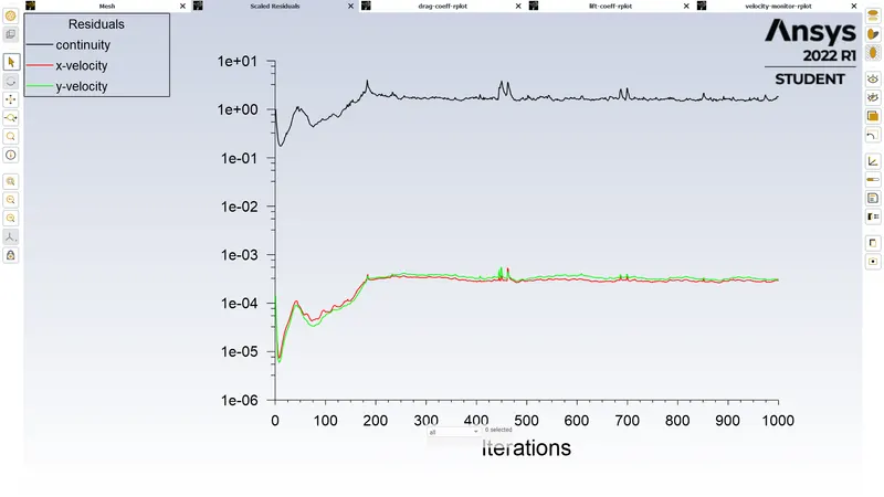
- The residuals are not sufficient for guaranting any form of convergence for this simulation. As a result, we observe the force parameters such as the coefficients of the lift and drag and the velocity at a point behind the cylinder.
- From the steady oscillatory behavior of the lift coefficient and the velocity montior, we can conclude that the simulation has reached "convergence" for steady and unsteadyt simulations
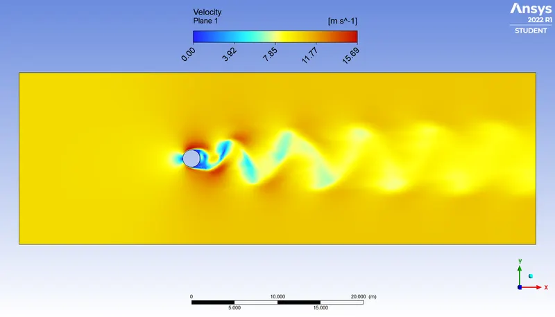
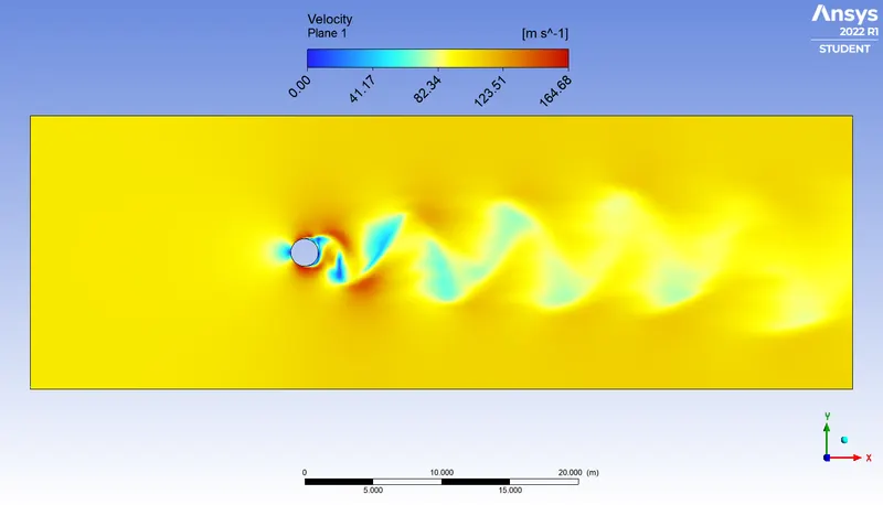
- From the velocity contours, we can observe the von-Karman vortex street has been successfully resolved.
From the reference "Numerical Simulation of Low Reynolds Number Fluid-Structure Interaction with Immersed Boundary Method", which also refers to various older study, we compare our numerical results for the coefficients of drag and lift.
| Case | Lift Coefficient | Drag Coefficient |
| Steady Re = 100 | 0.15 to -0.16 | 1.37 |
| Unsteady Re = 100 | 0.37 to -0.37 | 1.45 |
| Literature | 0.32 to -0.32 | between 1.33 and 1.38 |
From the reference "Numerical Study of Unsteady Flow around a Square Cylinder in Compare with Circular
Cylinder", we compare the Strohaul Number results
| Case | Strouhal Number |
| Unsteady Re = 100 | 0.167 |
| Literature | between 0.16 and 0.175 |
From the above validation study we can conclude that:
- The steady state analysis is useful to accurately capture the drag coefficient while performs poorly in resolving the variation of the lift coefficient.
- The unsteady analysis we observe that the obtained results are in 5% of the literature values hence unsteady analysis must be used for predicting oscillating motion of velocity and lift coefficient compared to the steadty state analysis.
- The Strohaul number obtained from the unsteady analysis is properly resolved as per the values available in the literature.
Steady State analysis of Re 10, 100, 1000, 10000, 100000:
In this section, we will carry out the steady state analysis for several Reynolds number for the flow over cylinder problem and determine the values for the coefficient of the lift and drag. For all the Reynolds number considered in this analysis, the flow is laminar accoriding to the theory. Hence, the laminar model are used for modeling the viscosity of the fluids. The setup for the current runs are identical to the one dicsussed in the simulation setup section. The Reynolds number for these simulations is modified by keeping the density and the dynamic viscosity as 1 kg/m3 and 0.02 kg/ms respectively and modifiying the inlet velocity. (For instance, for the current geometry to obtain a Reynolds number of 1000, we provide an inlet velocity of 10 m/s.)
The simulations are run till it is observed that the monitors for the lift and drag coefficient and the velocity monitor behind the cylinder have reached an approximate oscillating periodic motion or steady state.
Reynolds Number = 10
- Residuals vs the number of iterations
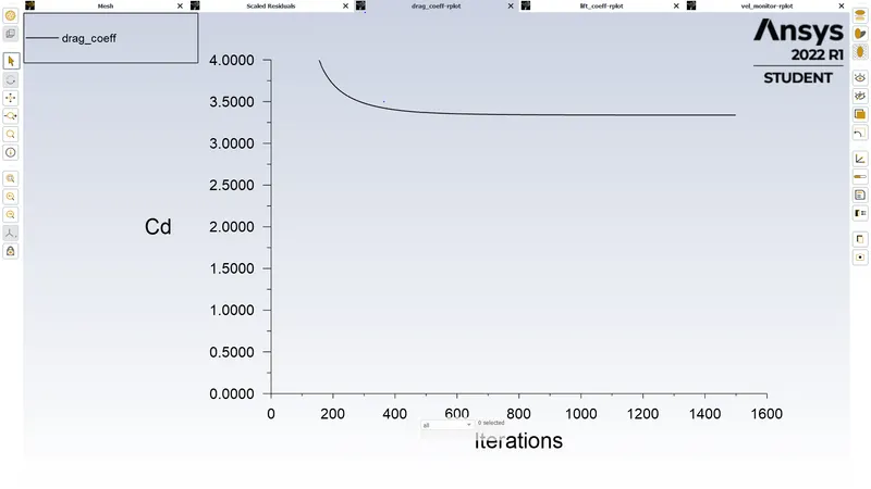
- Drag Coefficient vs the number of iterations
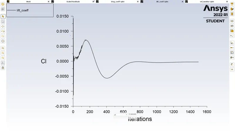
- Lift coefficient vs the number of iterations
- Velocity monitior vs number of iterations
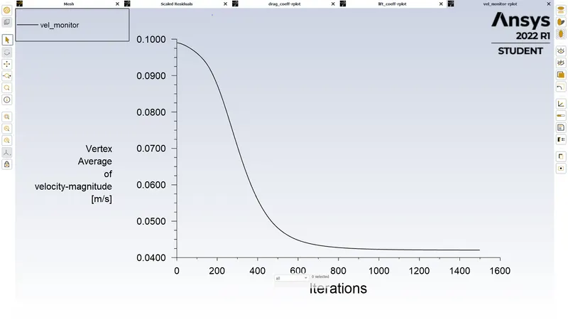
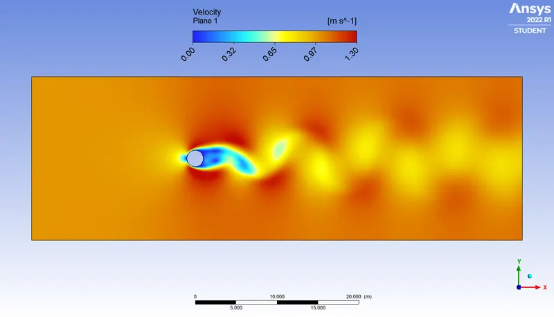
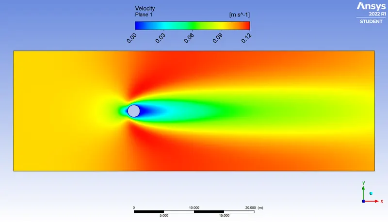
- Velocity contour for visualizing the flow (no vortex shedding is observed)
Reynold Number 100
- Residuals vs the number of iterations
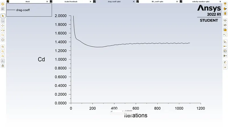
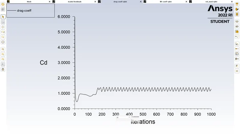
- Drag coefficient vs number of iterations
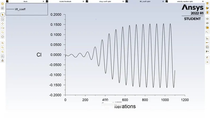
- Lift coefficient vs the number of iterations
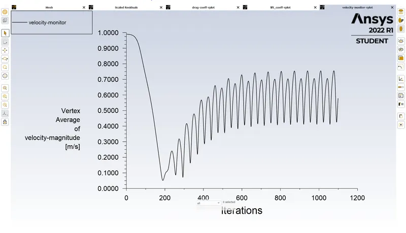
- Velocity monitor vs number of iterations
- Velocity contour to visualize the flow (vortex shedding is observed)
Reynolds Number 1000
- Residuals vs the number of iterations
- Drag coefficient vs number of iterations
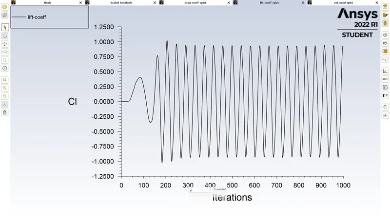
- Lift coefficient vs number of iterations
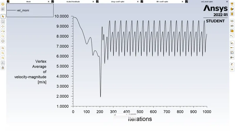
- Velocity monitor vs number of iterations
- Velocity contour to visualize the flow (vortex shedding is observed)
Reynolds Number 10000
- Residuals vs number of iterations
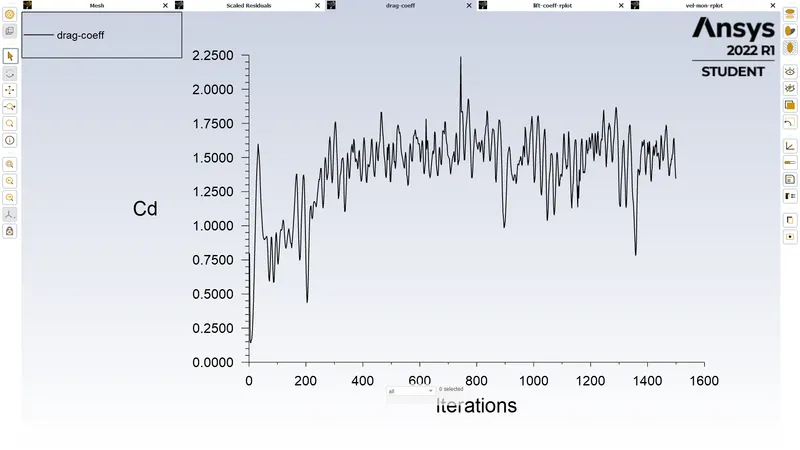
- Drag coefficient vs number of iterations
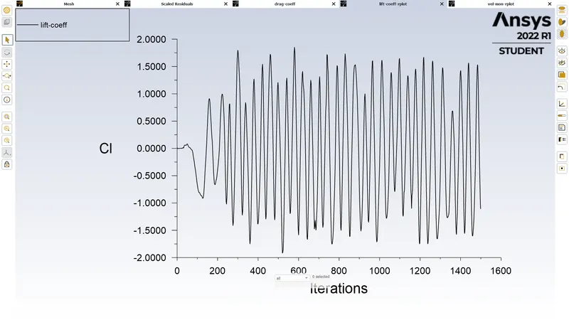
- Lift coefficient vs number of iterations
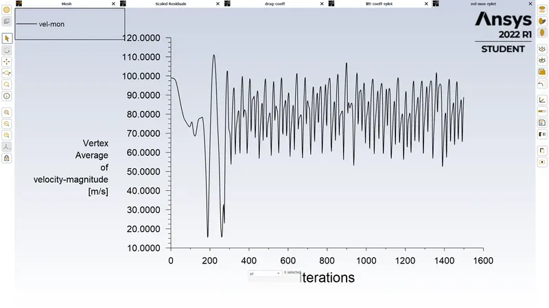
- Velocity monitor vs number of iterations
- Velocity contour to visualize the flow (vortex shedding is observed)
Reynolds Number 100000
- Residuals vs number of iterations
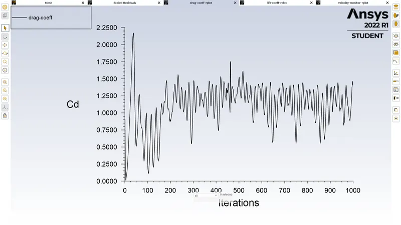
- Drag coefficient vs number of iterations
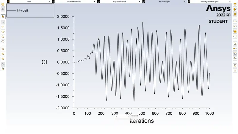
- Lift coefficient vs number of iterations
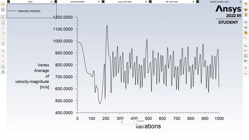
- Velcoity monitor vs number of iterations
- Velocity contour to visualize the flow (vortex shedding is observed)
We summarize the results of the drag and lift coefficient observed for the aforementioned simulation runs.
| Cases | Drag coefficient | Lift coefficient |
| Re = 10 | 3.34 | -0.00026 |
| Re = 100 | 1.37 | 0.15 to -0.16 |
| Re = 1000 | 1.15 | 0.93 to -0.93 |
| Re = 10000 | 1.25 | 1.5 to -1.5 |
| Re = 100000 | 1.28 | 1.25 to -1.16 |
The observed values are validated with the reference "https://kdusling.github.io/teaching/Applied-Fluids/DragCoefficient.html". Hence, we can say that even for the current mesh which definately coarse for the Higher Reynolds number of the study produce statistically significant results.
From the above plots, contour and table we make the following observations and conclusions
- No vortex shedding is observed for Reynolds number 10 and the phenomenon is present producing the von-Karman vortex street for the rest of the reynolds number. This observation is inline with the theoritical and experimental data.
- The "convergence" is observed in form of periodic oscillation of the lift coefficient and the velocity monitor for the Reynolds number for which vortex shedding is present.
- The Drag number decreases for Reynolds number 1000 and then almost becomes constant with no significant increase in the drag coefficient. This is very good indicator that the current simulations provide statistically significant results as they are very much inline with the experimental observations (5 % error margin)
- As the Reynolds number increases, we observe that the periodic motion of the lift and velocity monitor becomes random and even the drag coefficient becomes periodic and random. This suggests that the current mesh is not very suitable for high reynolds number studies and finer mesh should be used for those cases.
Conclusions:
From this study, we have explained the importance of the flow over a cylinder problem as it proves to be a simple model to understand the vortex shedding phenonemon. We have provide brief introduction to the theory relating to nondimensional parameters like Reynolds Number and Strouhal Number, origins of von-Karman vortex street and coefficients for quantifying the external flows' effectsd over blunt bodies. We have sucessfully carried out simulations for various Reynolds number and validated the results obtained using experimental and theoritical data.
References:
- Numerical Simulation of Low Reynolds Number Fluid-Structure Interaction with Immersed Boundary Method
- Numerical Study of Unsteady Flow around a Square Cylinder in Compare with Circular
Cylinder - https://kdusling.github.io/teaching/Applied-Fluids/DragCoefficient.html