Week 11 - Simulation of Flow through a pipe in OpenFoam

Aim:

Transient Simulation of the flow through the pipe at Reynolds Number 2100 and verification of the simulation results with the Hagen-Poiseuille flow.

Assumptions & Simplifications:

The reason for wedge shaped geometry simplification is as follows:

1. Simulating fluid flow through a 3D pipe is a computational expensive exercise, which poses a problem for practitioners who cannot avail high perfomance computing. To achieve our objectives, we exploit the axisymmetric nature of the cylindrical pipe. This simplification helps us to simulate the flow by just considering a small wedge instead of the entire geometry which degenerates the problem from three to two dimensions, which is computationally efficient technique.

The flow assumptions are as follows:

1. The flow is considered laminar, incompressible and steady (we carry out transient simulations and achieve the steady state results after simulating for a long period of time).
2. From the problem simplfication, the results obtained are two dimensional (The flow variations in the angular direction are neglected because their gradients vanish in the steady state).
3. The fluid properties such as dynamic viscosity `mu`, density `rho` and kinematic viscosity `nu` are considered to be invariant throughout the simulation.

Theory:

For steady fluid flow inside a pipe of constant cross-section, a pressure gradient is required along the length of the pipe. This physical law is termed as the Hagen-Poiseuille Law.

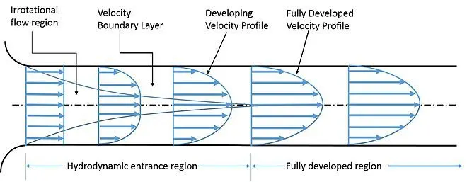
The derivations are done by using the above assumptions. The Navier-Stokes equation in the angular co-ordinates along the pipe length is as follows:

`1/r * {partial {r{ partial U}/{partial r}}}/{partial r} = 1/mu {dp}/{dx}`

Integrating the PDE we get the following formulaes for `{partial U}/{partial r}` and `U` and using appropriate boundary conditions at the wall and the centerline, where `G = {dp}/{dx}`

`{partial U}/{partial r} = -{Gr}/{2mu}`

`U = G/{4mu}(R^2 - r^2)`

Using simple manipulations on the above derived formulas, we can show the following mathematical equations hold true for the pipe flow

`v_{avg} = v_{max}/2`

`{dp}/{dx} = {8muu_{avg}piR^2}/{pi R^4}`

`mu{ {partial U}/{partial r}}|_{r=R} = -{GR}/2`

The above equations will be used to validate the simulation results

Problem Definition:

Reynolds Number `Re` = 2100

Diameter of the pipe `D` = 0.01 `m`

Kinematic viscosity of the fluid `nu` = `10^(-6) \ \ m^{2}/s`

Dynamic viscosity of the fluid `mu` = 0.00089 `Pa*s`

Density of the fluid `rho = {mu}/{nu}` = 890 `{kg}/m^{3}`

Development length for flow in pipe `L_{ent}` = `0.0575*Re*D` = 1.2075 `m`

Length of the pipe considered `L = L_{ent} + 0.3` ~ 1.5 `m`

Inlet Velocity = Average Velocity `v_{avg} = {Re*nu}/D` = 0.21 `m/s`

Wedge angle `theta` = 4

Setting up the OpenFOAM simulation files:

• The geometrical parameters such as the length of the pipe `L`, the diameter of the pipe `D`, the wedge angle `theta` and the mesh parameters such as the meshing in the axial `n_L` and the radial directions `n_D` (azimuthal direction meshing is not considered because we are solving a two dimensional flow) and the simple grading in those directions are the important features which will have a direct impact on the simulation results. Since, manual manipulating these features in the system/blockMeshDict file is physically exhausting task, we automate the file generation process using MATLAB. These automation will be essential for efficiently carrying out optimization studies.

%%

clear
close all
clc
%% Defining the fluid and flow properties

theta = input('Enter the value of the wedge angle (should be < 5)'); %Wedge angle
theta = theta*pi/180;
Re = 2100;   % Reynolds Number
D = 0.01;     % Diameter of the pipe
R = D/2;      % Radius of the pipe
L_e = 0.0575*Re*D; % Development length
L = L_e + 0.3;    % Length of the pipe

%% Defining inputs to the blockMeshDict file

% Defining the conversion paramerter
con = 1;

% Defining the six vertices
v0 = [0 0 0];
v1 = [L 0 0];
v2 = [L R*cos(-theta) R*sin(-theta)];
v3 = [0 R*cos(-theta) R*sin(-theta)];
v4 = [L R*cos(theta) R*sin(theta)];
v5 = [0 R*cos(theta) R*sin(theta)];


% Defining the number of cells and grading in the direction
nx = 200; % Axial dir
ny = 50;  % Radial dir
nz = 1;   % Azimuthal dir

sgx = 1;
sgy = 0.2;
sgz = 1;

% header lines
h1 = '/*--------------------------------*- C++ -*----------------------------------*\';
h2 = ' =========                 |';
h3 = ' \\      /  F ield         | OpenFOAM: The Open Source CFD Toolbox';
h4 = '  \\    /   O peration     | Website:  https://openfoam.org';
h5 = '   \\  /    A nd           | Version:  9';
h6 = '    \\/     M anipulation  |';
h7 = '\*---------------------------------------------------------------------------*/';
h8 = 'FoamFile';
h9 = '{';
h10 = '     format      ascii;';
h11 = '     class       dictionary;'; 
h12 = '     object      blockMeshDict;';     
h13 = '}';
h14 = '// * * * * * * * * * * * * * * * * * * * * * * * * * * * * * * * * * * * * * //';

% tail lines
h15 = '// ************************************************************************* //';

%% Writing in the blockMeshDict file

fh = fopen('blockMeshDict.txt','w');

fprintf(fh,'%s\n',h1);
fprintf(fh,'%s\n',h2);
fprintf(fh,'%s\n',h3);
fprintf(fh,'%s\n',h4);
fprintf(fh,'%s\n',h5);
fprintf(fh,'%s\n',h6);
fprintf(fh,'%s\n',h7);
fprintf(fh,'%s\n',h8);
fprintf(fh,'%s\n',h9);
fprintf(fh,'%s\n',h10);
fprintf(fh,'%s\n',h11);
fprintf(fh,'%s\n',h12);
fprintf(fh,'%s\n',h13);
fprintf(fh,'%s\n',h14);

fprintf(fh,'\n');
fprintf(fh,'%s %f\n','convertToMeters',con);
fprintf(fh,'\n');

fprintf(fh,'%s\n','vertices');
fprintf(fh,'%s\n','(');
fprintf(fh,'%s (%f %f %f)\n',blanks(4),v0(1),v0(2),v0(3));
fprintf(fh,'%s (%f %f %f)\n',blanks(4),v1(1),v1(2),v1(3));
fprintf(fh,'%s (%f %f %f)\n',blanks(4),v2(1),v2(2),v2(3));
fprintf(fh,'%s (%f %f %f)\n',blanks(4),v3(1),v3(2),v3(3));
fprintf(fh,'%s (%f %f %f)\n',blanks(4),v4(1),v4(2),v4(3));
fprintf(fh,'%s (%f %f %f)\n',blanks(4),v5(1),v5(2),v5(3));
fprintf(fh,'%s\n',');');
fprintf(fh,'\n');

fprintf(fh,'%s\n','blocks');
fprintf(fh,'%s\n','(');
fprintf(fh,'%s %s (%d %d %d %d %d %d %d %d) %s (%d %d %d) %s (%f %f %f)\n',...
        blanks(4),'hex',0,1,2,3,0,1,4,5,blanks(1),nx,ny,nz,'simpleGrading',...
        sgx,sgy,sgz);
fprintf(fh,'%s\n',');');
fprintf(fh,'\n');

fprintf(fh,'%s\n','edges');
fprintf(fh,'%s\n','(');
fprintf(fh,'%s\n',');');
fprintf(fh,'\n');

fprintf(fh,'%s\n','boundary');
fprintf(fh,'%s\n','(');
%inlet
fprintf(fh,'%s %s\n',blanks(4),'inlet');
fprintf(fh,'%s %s\n',blanks(4),'{');
fprintf(fh,'%s %s %s\n',blanks(8),'type','patch;');
fprintf(fh,'%s %s\n',blanks(8),'faces');
fprintf(fh,'%s %s\n',blanks(8),'(');
fprintf(fh,'%s (%d %d %d %d)\n',blanks(12),0,5,3,0);
fprintf(fh,'%s %s\n',blanks(8),');');
fprintf(fh,'%s %s\n',blanks(4),'}');
%outlet
fprintf(fh,'%s %s\n',blanks(4),'outlet');
fprintf(fh,'%s %s\n',blanks(4),'{');
fprintf(fh,'%s %s %s\n',blanks(8),'type','patch;');
fprintf(fh,'%s %s\n',blanks(8),'faces');
fprintf(fh,'%s %s\n',blanks(8),'(');
fprintf(fh,'%s (%d %d %d %d)\n',blanks(12),1,2,4,1);
fprintf(fh,'%s %s\n',blanks(8),');');
fprintf(fh,'%s %s\n',blanks(4),'}');
%wedgeFront
fprintf(fh,'%s %s\n',blanks(4),'wedgeFront');
fprintf(fh,'%s %s\n',blanks(4),'{');
fprintf(fh,'%s %s %s\n',blanks(8),'type','wedge;');
fprintf(fh,'%s %s\n',blanks(8),'faces');
fprintf(fh,'%s %s\n',blanks(8),'(');
fprintf(fh,'%s (%d %d %d %d)\n',blanks(12),0,1,4,5);
fprintf(fh,'%s %s\n',blanks(8),');');
fprintf(fh,'%s %s\n',blanks(4),'}');
%wedgeBack
fprintf(fh,'%s %s\n',blanks(4),'wedgeBack');
fprintf(fh,'%s %s\n',blanks(4),'{');
fprintf(fh,'%s %s %s\n',blanks(8),'type','wedge;');
fprintf(fh,'%s %s\n',blanks(8),'faces');
fprintf(fh,'%s %s\n',blanks(8),'(');
fprintf(fh,'%s (%d %d %d %d)\n',blanks(12),0,3,2,1);
fprintf(fh,'%s %s\n',blanks(8),');');
fprintf(fh,'%s %s\n',blanks(4),'}');
%wall
fprintf(fh,'%s %s\n',blanks(4),'wall');
fprintf(fh,'%s %s\n',blanks(4),'{');
fprintf(fh,'%s %s %s\n',blanks(8),'type','wall;');
fprintf(fh,'%s %s\n',blanks(8),'faces');
fprintf(fh,'%s %s\n',blanks(8),'(');
fprintf(fh,'%s (%d %d %d %d)\n',blanks(12),5,4,2,3);
fprintf(fh,'%s %s\n',blanks(8),');');
fprintf(fh,'%s %s\n',blanks(4),'}');
%centerline
fprintf(fh,'%s %s\n',blanks(4),'centerline');
fprintf(fh,'%s %s\n',blanks(4),'{');
fprintf(fh,'%s %s %s\n',blanks(8),'type','empty;');
fprintf(fh,'%s %s\n',blanks(8),'faces');
fprintf(fh,'%s %s\n',blanks(8),'(');
fprintf(fh,'%s (%d %d %d %d)\n',blanks(12),0,1,1,0);
fprintf(fh,'%s %s\n',blanks(8),');');
fprintf(fh,'%s %s\n',blanks(4),'}');
fprintf(fh,'%s\n',');');
fprintf(fh,'\n');

fprintf(fh,'%s\n','mergePatchPairs');
fprintf(fh,'%s\n','(');
fprintf(fh,'%s\n',');');
fprintf(fh,'\n');

fprintf(fh,'%s\n',h15);

fclose(fh);

/*--------------------------------*- C++ -*----------------------------------*\
 =========                 |
 \\      /  F ield         | OpenFOAM: The Open Source CFD Toolbox
  \\    /   O peration     | Website:  https://openfoam.org
   \\  /    A nd           | Version:  9
    \\/     M anipulation  |
\*---------------------------------------------------------------------------*/
FoamFile
{
     format      ascii;
     class       dictionary;
     object      blockMeshDict;
}
// * * * * * * * * * * * * * * * * * * * * * * * * * * * * * * * * * * * * * //

convertToMeters 1.000000

vertices
(
     (0.000000 0.000000 0.000000)
     (1.507500 0.000000 0.000000)
     (1.507500 0.004997 -0.000174)
     (0.000000 0.004997 -0.000174)
     (1.507500 0.004997 0.000174)
     (0.000000 0.004997 0.000174)
);

blocks
(
     hex (0 1 2 3 0 1 4 5)   (200 50 1) simpleGrading (1.000000 0.200000 1.000000)
);

edges
(
);

boundary
(
     inlet
     {
         type patch;
         faces
         (
             (0 5 3 0)
         );
     }
     outlet
     {
         type patch;
         faces
         (
             (1 2 4 1)
         );
     }
     wedgeFront
     {
         type wedge;
         faces
         (
             (0 1 4 5)
         );
     }
     wedgeBack
     {
         type wedge;
         faces
         (
             (0 3 2 1)
         );
     }
     wall
     {
         type wall;
         faces
         (
             (5 4 2 3)
         );
     }
     centerline
     {
         type empty;
         faces
         (
             (0 1 1 0)
         );
     }
);

mergePatchPairs
(
);

// ************************************************************************* //

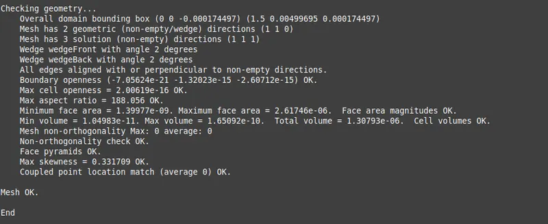
• The mesh generated from the above procedure is validated by using the command checkMesh in the terminal and checking the angle made by the wedges with the principle y-axis.

• After validating the mesh, we set the initial conditions 0/p (pressure) and 0/U (velocity) files as per the problem definition and appropriate boundary conditions.

/*--------------------------------*- C++ -*----------------------------------*\
  =========                 |
  \\      /  F ield         | OpenFOAM: The Open Source CFD Toolbox
   \\    /   O peration     | Website:  https://openfoam.org
    \\  /    A nd           | Version:  9
     \\/     M anipulation  |
\*---------------------------------------------------------------------------*/
FoamFile
{
    format      ascii;
    class       volScalarField;
    object      p;
}
// * * * * * * * * * * * * * * * * * * * * * * * * * * * * * * * * * * * * * //

dimensions      [0 2 -2 0 0 0 0];

internalField   uniform 0;

boundaryField
{
    inlet
    {
        type            zeroGradient;
    }
    outlet
    {
        type            fixedValue;
        value		uniform 0;
    }
    wedgeFront
    {
        type            wedge;
    }
    wedgeBack
    {
        type            wedge;
    }
    wall
    {
    	type		zeroGradient;
    }
    centerline
    {
        type            empty;
    }
    
}

// ************************************************************************* //

/*--------------------------------*- C++ -*----------------------------------*\
  =========                 |
  \\      /  F ield         | OpenFOAM: The Open Source CFD Toolbox
   \\    /   O peration     | Website:  https://openfoam.org
    \\  /    A nd           | Version:  9
     \\/     M anipulation  |
\*---------------------------------------------------------------------------*/
FoamFile
{
    format      ascii;
    class       volVectorField;
    object      U;
}
// * * * * * * * * * * * * * * * * * * * * * * * * * * * * * * * * * * * * * //

dimensions      [0 1 -1 0 0 0 0];

internalField   uniform (0 0 0);

boundaryField
{
    inlet
    {
        type            fixedValue;
        value           uniform (0.21 0 0);
    }
    outlet
    {
        type            zeroGradient; 
    }
    wedgeFront
    {
        type            wedge;
    }
    wedgeBack
    {
        type            wedge;
    }
    wall
    {
       type 		fixedValue;
       value 		uniform (0 0 0);
    }
    centerline
    {
        type            empty;
    }
}

// ************************************************************************* //

• The value of the kinematic viscosity `nu` is set as per the problem definition in the constant/transportProperties file.

/*--------------------------------*- C++ -*----------------------------------*\
  =========                 |
  \\      /  F ield         | OpenFOAM: The Open Source CFD Toolbox
   \\    /   O peration     | Website:  https://openfoam.org
    \\  /    A nd           | Version:  9
     \\/     M anipulation  |
\*---------------------------------------------------------------------------*/
FoamFile
{
    format      ascii;
    class       dictionary;
    location    "constant";
    object      transportProperties;
}
// * * * * * * * * * * * * * * * * * * * * * * * * * * * * * * * * * * * * * //

nu              [0 2 -1 0 0 0 0] 1e-6;


// ************************************************************************* //

• The solver is set as icoFoam with total simulation time set as 14 which equates to two passes of the fluid element through the computational domain, thereby assuring the results obtained by the transient solver are in steady state. We set the the time step as `10^(-3)`

/*--------------------------------*- C++ -*----------------------------------*\
  =========                 |
  \\      /  F ield         | OpenFOAM: The Open Source CFD Toolbox
   \\    /   O peration     | Website:  https://openfoam.org
    \\  /    A nd           | Version:  9
     \\/     M anipulation  |
\*---------------------------------------------------------------------------*/
FoamFile
{
    format      ascii;
    class       dictionary;
    location    "system";
    object      controlDict;
}
// * * * * * * * * * * * * * * * * * * * * * * * * * * * * * * * * * * * * * //

application     icoFoam;

startFrom       latestTime;

startTime       0;

stopAt          endTime;

endTime         14;

deltaT          1e-3;

writeControl    timeStep;

writeInterval   2.5e3;

purgeWrite      0;

writeFormat     ascii;

writePrecision  6;

writeCompression off;

timeFormat      general;

timePrecision   6;

runTimeModifiable true;


// ************************************************************************* //

Simulation Results:

After setting up the problem, we solve it by providing the command icoFoam on the terminal. The contours and the plots of various flow parameters are given below and the observations related to them are noted in the next section

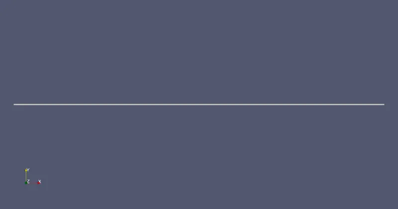
The computational domain along the pipe length (along the x-direction):

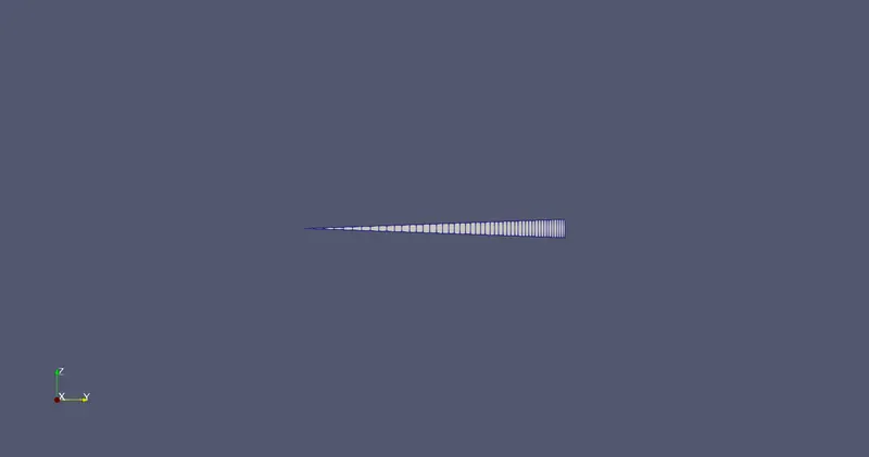
The computational domain of the pipe cross section with simpleGrading near the walls for better resolution of the gradients (wedge in the y-z plane):

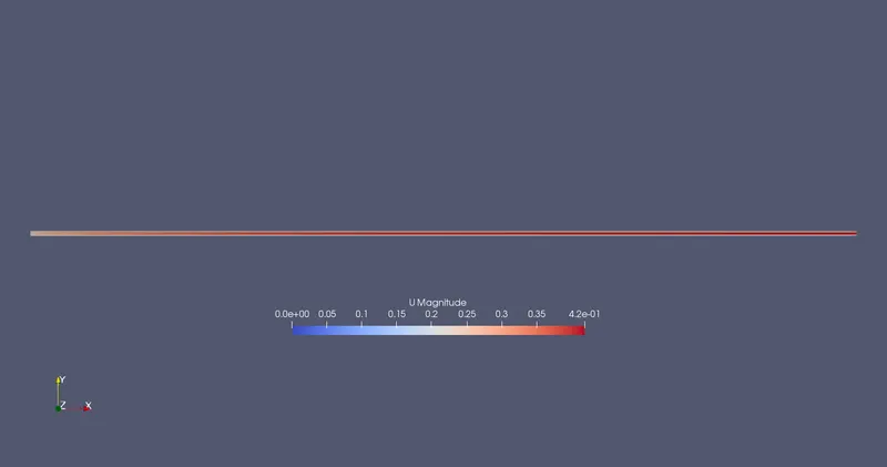
Velocity Contour at t= 14 (after using the Reflect filter):

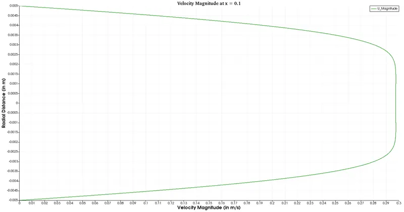
Velocity profile @ x = 0.1 from the inlet

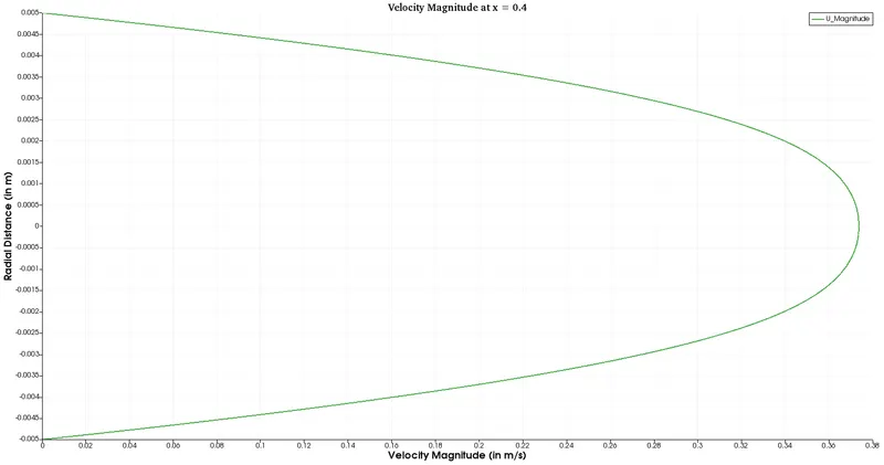
Velocity profile @ x = 0.4 from the inlet

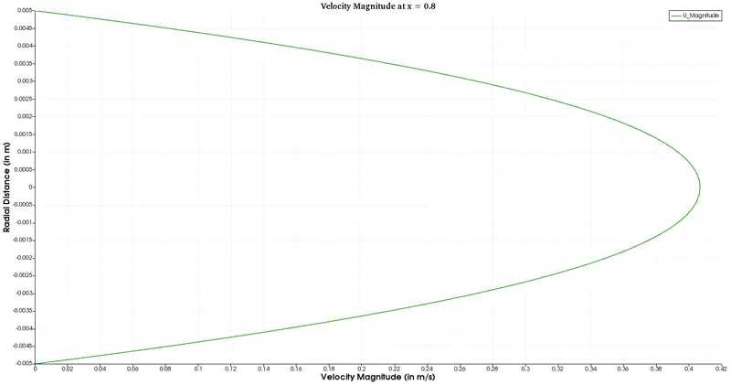
Velocity profile @ x = 0.8 from the inlet

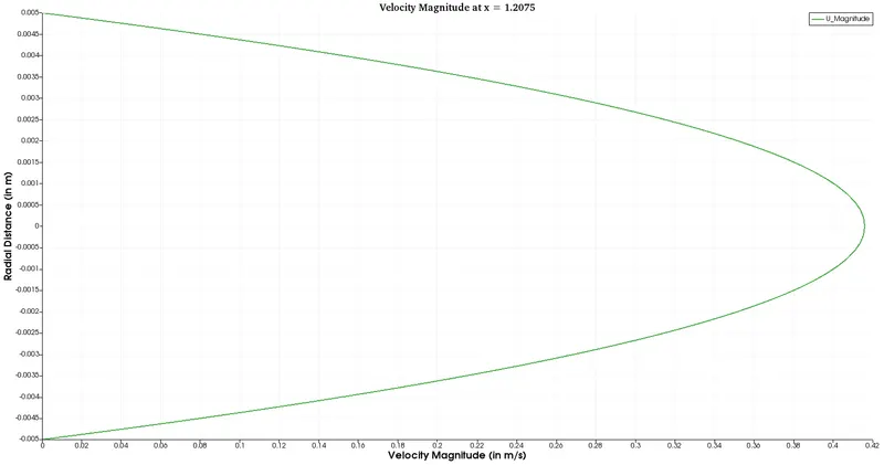
Velocity profile @ x = 1.2075 from the inlet (Theoritical Entrance length, flow is just completely developed)

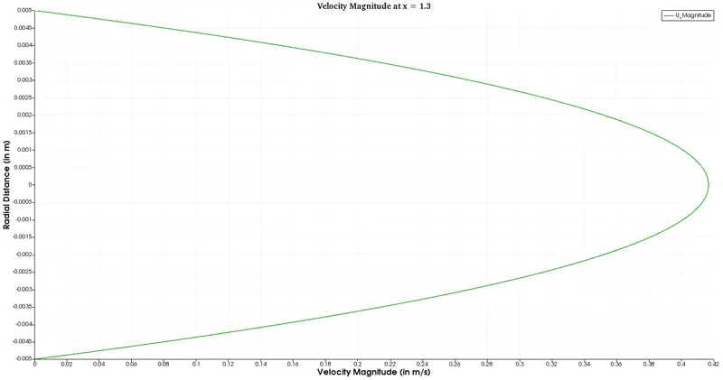
Velocity profile @ x = 1.3 from the inlet (Flow is completely developed)

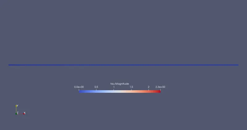
Using functionalities such as Calculators and Gradients of unstructured data in Paraview we can calculate the Shear stress in the entire domain.

Shear Stress Contour at t = 14 (after using the Reflect filter):

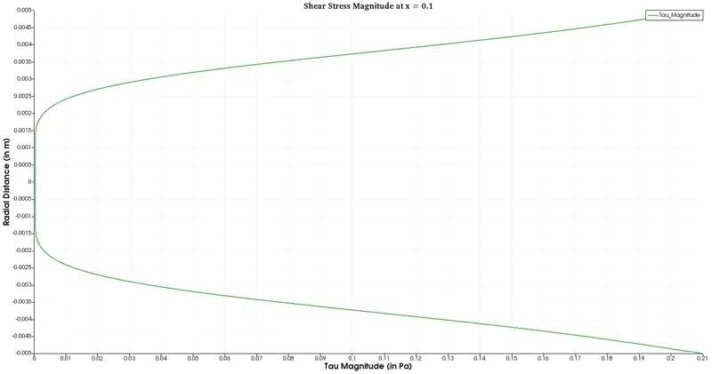
Shear Stress profile @ x = 0.1 from the inlet

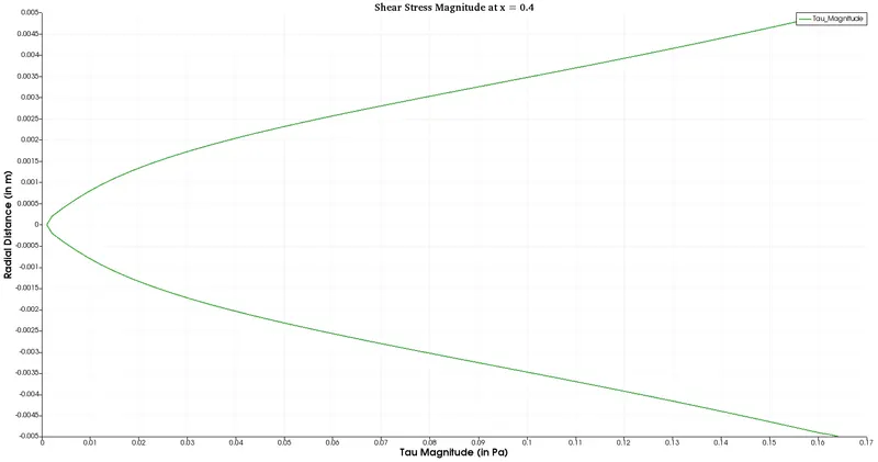
Shear Stress profile @ x = 0.4 from the inlet

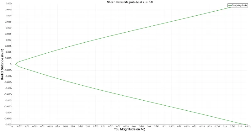
Shear Stress profile @ x = 0.8 from the inlet

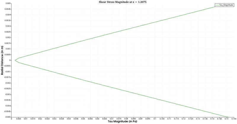
Shear Stress profile @ x = 1.2075 from the inlet (Theoritical Entrance Length)

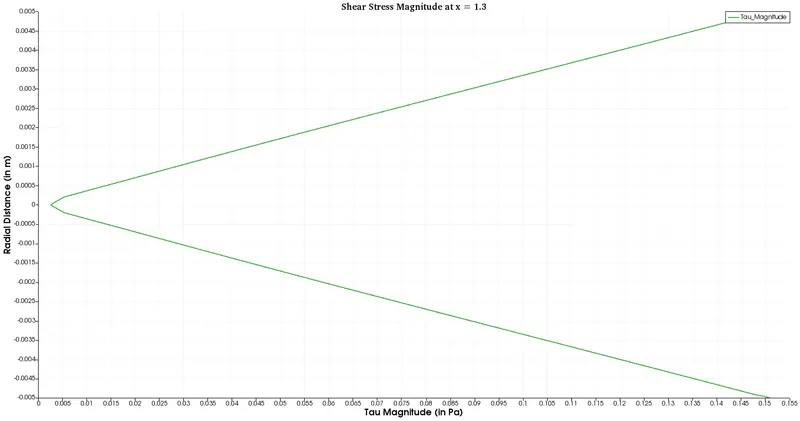
Shear Stress profile @ x=1.3 from the inlet (Flow is completely developed)

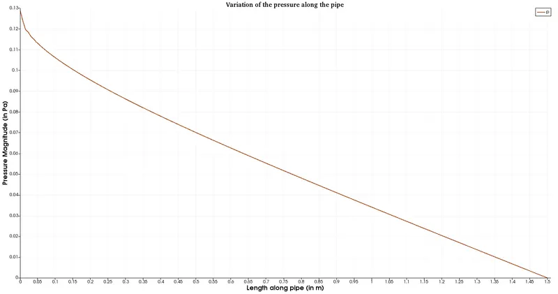
Pressure variation along the pipe length @ t=14:

Observations:

1. The velocity graphs before the entrance length `x < 1.2075` show considerable changes while for velocity graphs `x > 1.2075` are almost identical. This is physical trend as per the Hagen-Poiseuille theory, because boundary layers are still growing in developing regions.
2. The maximum velocity in all the velocity graph is at the centerline and is almost double the inlet velocity which is the average velocity in the domain.
3. Similarly, shear stress `tau` graph shows siginficant changes before reaching the entrance length and virtually no changes after it.
4. The pressure losses are non-linear in the developing region and linear in the developed region which is in accordance with the theoritical results.

Validation of the simulation results:

From the theory, we can calculate the the maximum value of the velocity, the pressure gradient and the shear stress and compare our simulation results to validate them.

Flow parameter	Theoritical Value	Simulation Value	Relative Error %
Maximum Velocity	0.42	0.418	0.48
Pressure Gradient	0.0672	0.0682	1.54
Max Shear Stress at the wall	0.1495	0.1507	1.34

Since the relative errors in these significant parameters are `< 5%`, we can conclude that the wedge geometry is a valid geometric simplification for simulating fluid flow in a pipe

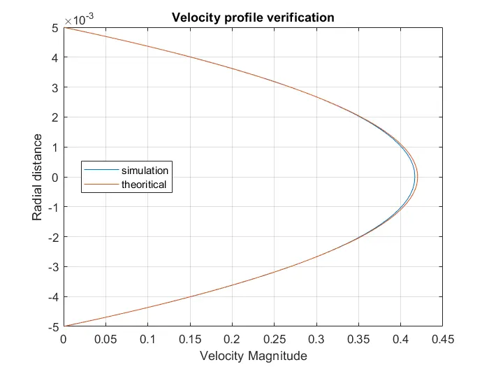
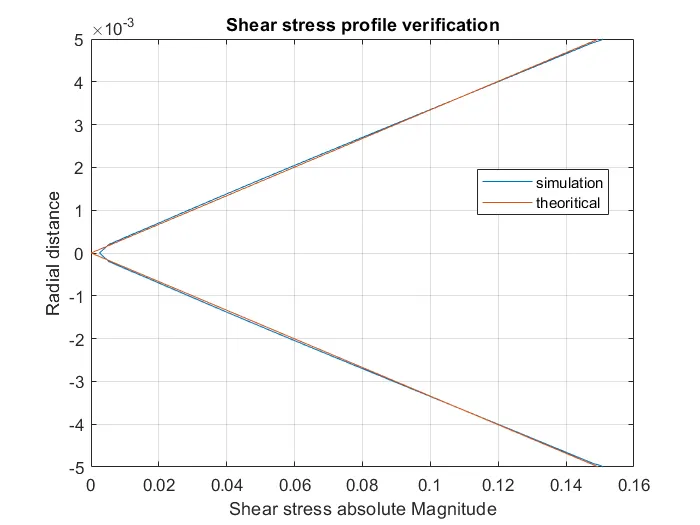
We validate the velocity and shear stress profile at the x = 1.2075 and compare it with theoritical results using following MATLAB code and data from the simulation results exported from Paraview. The results are almost identical further proving the correctness of the simulation

%%
clear
close all
clc

%% Reading the CSV file

opts = detectImportOptions('D:\Certification\images\dev_flow.csv');
mat = readmatrix('D:\Certification\images\dev_flow.csv',opts);
r = mat(:,15);
G = 59.8080;
mu = 0.00089;
R = 0.005;
vel_the = (G./(4.*mu)).*(R^2 - r.^2);
shear_the = abs(-G.*r/2);

figure(1)
plot(mat(:,7),r,vel_the,r)
legend('simulation','theoritical','Location','best')
grid on
xlabel('Velocity Magnitude')
ylabel('Radial distance')
title('Velocity profile verification')

figure(2)
plot(abs(mat(:,10)),r,shear_the,r)
legend('simulation','theoritical','Location','best')
grid on
xlabel('Shear stress absolute Magnitude')
ylabel('Radial distance')
title('Shear stress profile verification')