Week 9 - FVM Literature Review

Aim:

Define Finite Volume Method, point out the significant difference between the Finite Volume Method (FVM) and Finite Difference Method (FDM) and desrcibe the need of interpolation and flux limiter schemes in FVM.

Solution:

Definition of Finite Volume Method:

The Finite Volume Method is the integral form representation of the transport equations for fluid flow and heat transfer for a finite control volume. The most general form control volum formulation of the transport equation can be represented as follows. All the conservation equations related to fluid flow can be expressed in this format.

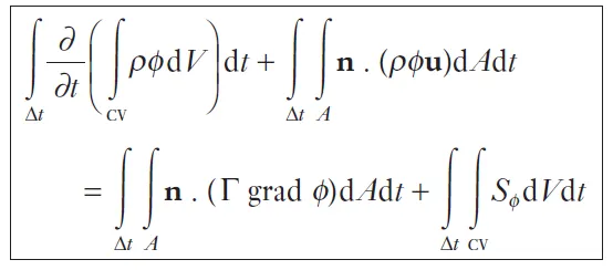
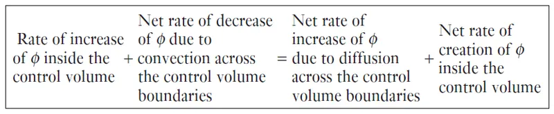
The integral form is essientially a conservation of the scalar or vector quantity `phi` inside the control volume. The LHS of the equation describes the temporal change of the value of `phi` inside the control volume and net decrease of `phi` due to convection. While, the RHS of the equation describes the effects of diffusion and source terms on `phi`. Mathematically, it can be represented as:

The transport equations can be solved by the FVM method using the following steps:

• Represent the transport equation into control volume intergral form and generating the computational grid of control volumes for the problem
• Discretize the equation into algebraic form
• Use linear solver to solve the system of algebraic equations with suitable representation of initial and boundary conditions. 

Difference between the Finite Volume Method and Finite Difference Method:

• One of the major difference between the FVM and FDM methods is the form in which the governing equations are represented. For the FVM, the transport equations are represented in the integral form (control volume integral form) while the FDM are implemented in the differential form of the transport equations (partial differential equation form).
• In the FVM, even after discretization the physical interpretation of the transport equation is conserved (the rate of change of value in the CV is equal to changes bought in by the fluxes and the source terms). On the other hand, the information of the PDE is not retained after discretization in FDM.
• FDM are generally popular for structured grids but are difficult to implement on curved boundaries. The FVM method is valid for any shape of control volume and as a result can be used to make unstructured grids for complex geometries.

Interpolation Schemes:

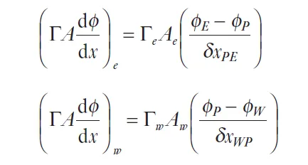
In the FVM formulation we observe that values of the variable `phi` and its gradient are required because of the flux on the control surface of the cell volume. For interpolating the information available at the cell centers to the surface of the control volume we require the interpolation schemes.

For instance, in the 1D heat conduction equation, the gradients of the temperature at the surface are obtained by linear interpolation between the cell centers.

For convective terms, several interpolation techniques are available and their success depends upon the satisfaction of the four important criteria:

• Conservativeness (Representation of the flux in a consistent manner)
• Boundedness 
• Transportivness
• Accuracy (Order of the scheme derived from the Talyor series discretisation error)

Few of the important schemes are as follows:

1. Central differencing scheme: It has conservative property but does not have boundness for Pe > 2 and does not account for transportivness (influence of the flow direction).
2. Upwind Scheme: It properly satisfies the conservative, boundedness and transportivness properties but has low order of accuracy which leads to numerical diffusion in problems with sharp interfaces
3. Hybrid differencing scheme: It is a combination of the Central differencing scheme and the upwind scheme depending on the Peclet number. Still faces the low order of accuracy issue as Upwind scheme. Power law sheme has almost the same behaviour.
4. QUICK scheme (Quadractic Upwind Interpolation for Convective Kinetics): It is a scheme which satisfies all the four properties of conservativness, boundedness, transportivness and has a 3rd order accuracy because of its quadratic nature. The scheme is conditionally stable and as a result contains artificial wiggles which can lead to spuriors results.

Flux Limiters:

To address the issue of unphysical oscillatory behaviour of the higher order schemes, we introduce the concept of flux limiters. The concept behind the Total variation diminishing (TVD) or flux limiters schemes, is to introduce an artificial diffusion fragment or weighting towards the upstream contribution.

Mathematically, they can be represented as follows

`phi_e = phi_P + 1/2psi(r)(phi_E - phi_P)`,

where,

`r = {phi_P - phi_W}/{phi_E - phi_P}`

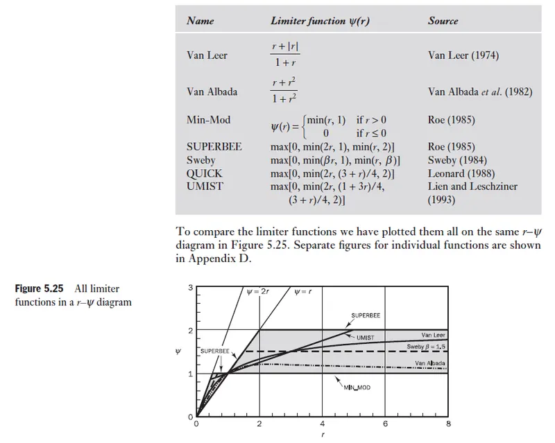
For constructing a second order TVD scheme, the criteria laid down by Sweby should be satisified. The schemes are shown below