Week 6: Conjugate Heat Transfer Simulation

Aim:

Simulate conjugate heat transfer model of flow through a pipe.

Objectives:

• Designing a duct with wall thickness using CONVERGE Studio.
• Setting up the conjugate heat transfer case using CONVERGE Studio.
• Carrying out a grid dependence study and selecting the appropriate mesh for the simulation.
• Documenting the effects of the supercycle stage interval.

Geometry:

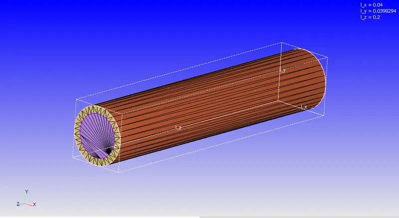
The geometry used for the modelling a duct is an annular cylinder with the inner diameter as 0.03 m and outter diameter set to 0.04 m. The length of the pipe is equal to 0.2 m. After generating the geometry, we run a diagnostic check to validate the correctness of the geometry and then flag the boundaries of the model with appropriate flags.

The final pre-processed model of the duct is illustrated below

Case Setup:

The case setup tree is populated using the following settings using the CONVERGE Studio GUI

• Application Type subtree:
  • Since we are tackling a general transient flow problem, a time based application is chosen in the cuurent study
• Materials subtree:
  • In the current simulation, we setup a gas + solid simulation and choose standard air as the working fluid and aluminium as the working solid
  • The default gas, solid and global transport properties are chosen for the simualtion
• Simulation parameters subtree:
  • A fully hydrodynamic transient simualtion using compressible gas flow solver is chosen for the current study
  • The total simulation time is set to 0.5 seconds and the time step is set to variable time stepping algortihm based on the CFL criteria
  • The default Navier-Stokes solver is chosen for the study
• Boundary Conditions subtree:
  • Outer Wall: Velocity = (Not applicable since no contact with fluid), Temperature = Heat flux of `10{-4} W/m^{2}`
  • Side Thickness Wall: Velocity = (Not applicable since no contact with fluid), Temperature = zero normal gradient
  • Inlet: Pressure = zero normal gradient, Velocity = 7.35 m/s (For Reynolds Number = 7000), Temperature = 300K, Species = Standard Air, Turbulent Kinetic Energy and Turbulent Dissipation = default values
  • Outlet: Pressure = Fixed Value of 101325 Pa (1 atm), Velocity = zero normal gradient, Temperature, species, turbulent kinetic energy and turbulent dissipation = Backflow
  • Interface: Forward side is in contact with the fluid, Velocity, Temperature, turbulent dissipation = law of the wall and turbulent kinetic energy = zero normal gradient. Reverse side is in contact with the solid, Velocity = (Not applicable since no contact with fluid), Temperature Boundary condition = specified value from the forward side.
• Initial Conditons and events subtree:
  • The fluid domain is initialized with stationary air at 300K with the pressure values 101325 Pa and the solid domain is initialized with aluminium at 300K
• Physical Models subtree:
  • A standard RNG RANS turbulence model was chosen for the simulation
  • Super cycling model was chosen for with data storing starting at 0.05 s and time length of the stage as 0.05 seconds for the grid dependence study.
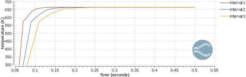
  • For understanding the effects of the super cycle interval, we vary the time length of the stage as 0.01, 0.02 and 0.03
• Grid Control
  • For the grid dependence study, we choose the base grid as 0.004, 0.003 and 0.002m as coarse, fine and finer mesh respectively

Grid Dependence Study & Supercycle interval Study:

The contours and line plots of flow properties are as follows:

Mesh 1: Animation Link

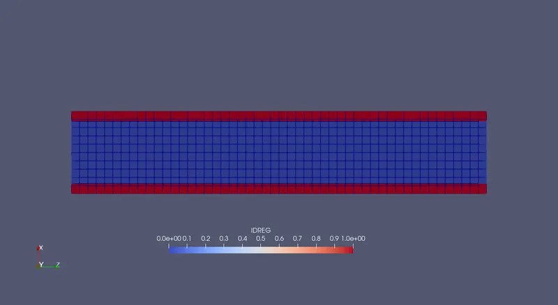
Mesh with both the streams/regions visible

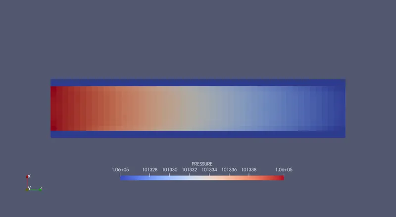
Pressure contour @ t - 0.5 seconds

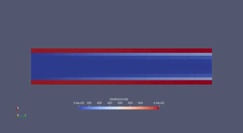
Temperature contour @ t - 0.5 seconds

Velocity Contour @ t - 0.5 seconds

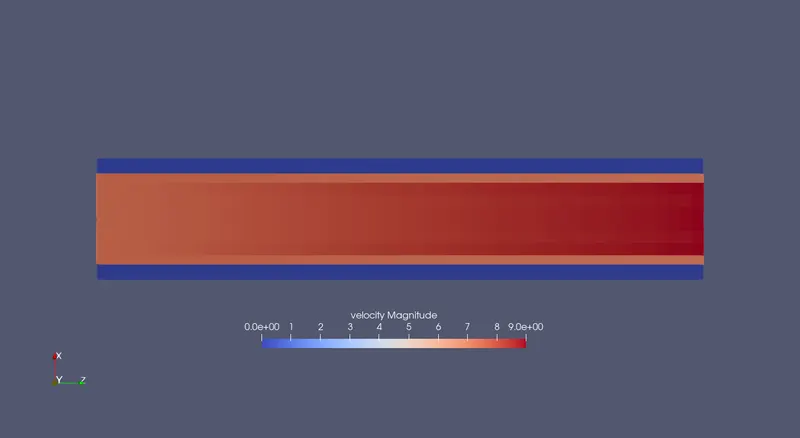
Yplus contour @ t - 0.5 seconds

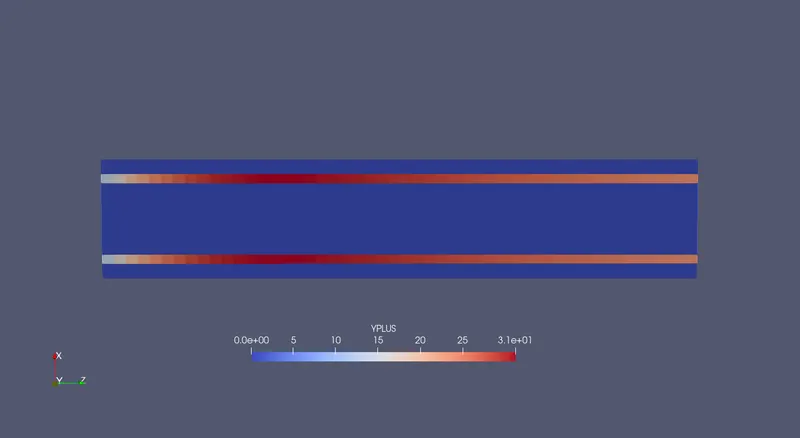
Mesh 2: Animation Link

Mesh with both the streams/regions visible

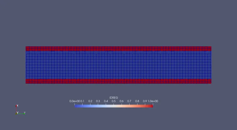
Pressure contour @ t - 0.5 seconds

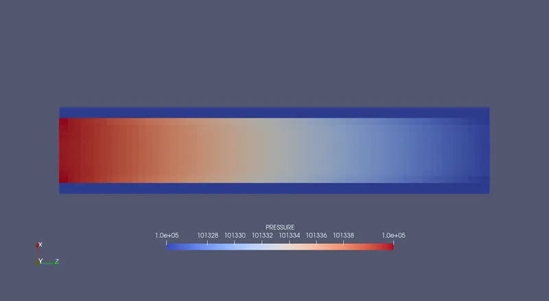
Temperature contour @ t - 0.5 seconds

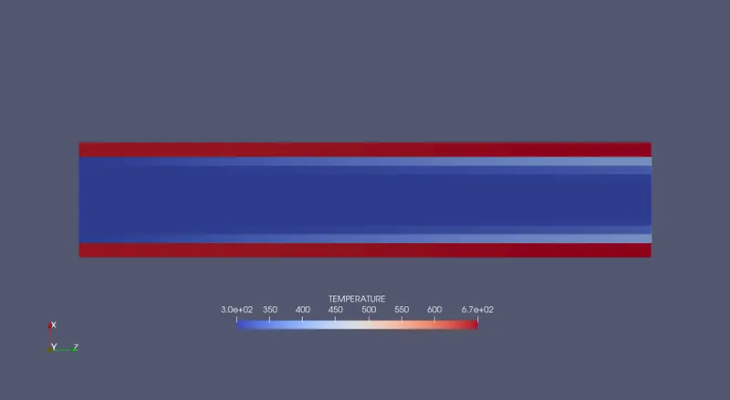
Velocity Contour @ t - 0.5 seconds

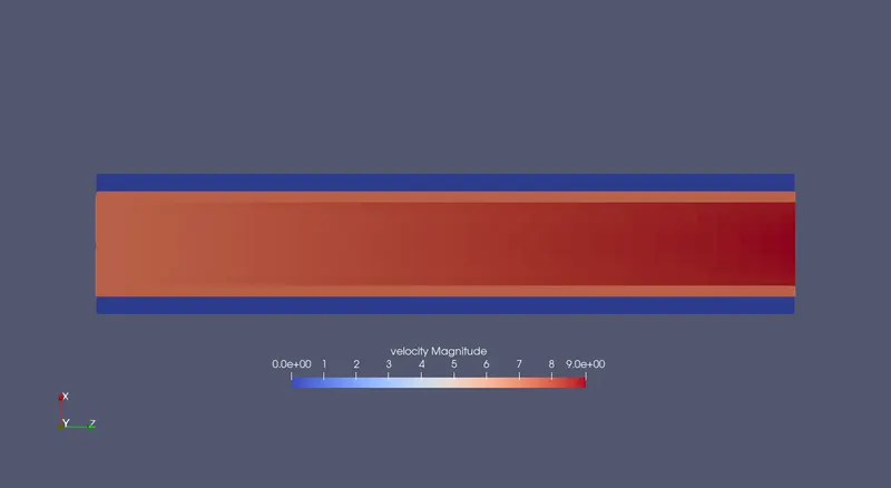
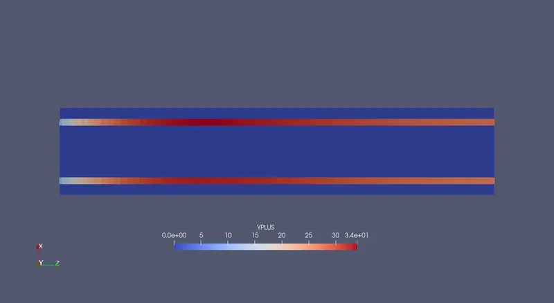
Yplus contour @ t - 0.5 seconds

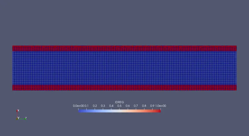
Mesh 3: Animation Link

Mesh with both the streams/regions visible

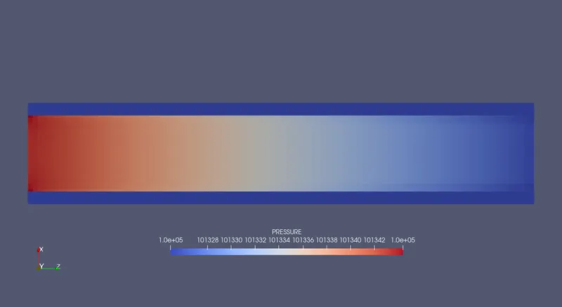
Pressure contour @ t - 0.5 seconds

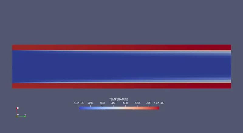
Temperature contour @ t - 0.5 seconds

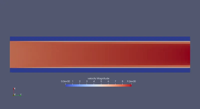
velocity contour @ t - 0.5 seconds

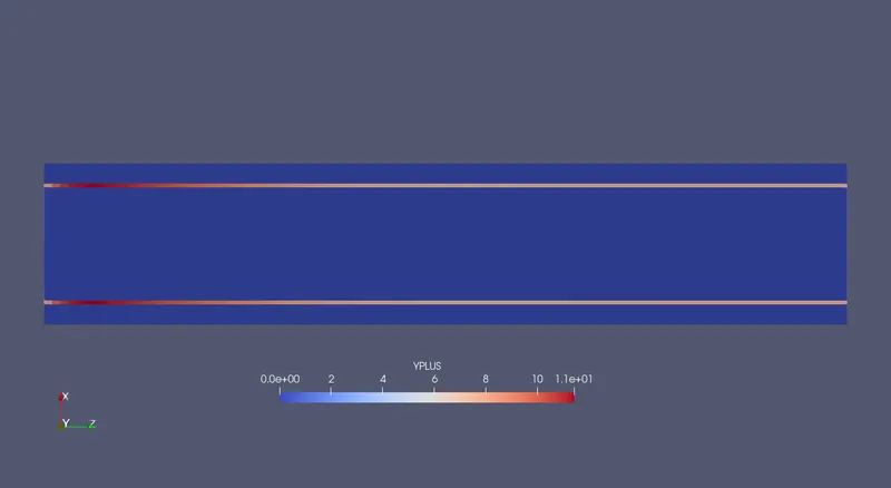
Yplus contour @ t - 0.5 seconds

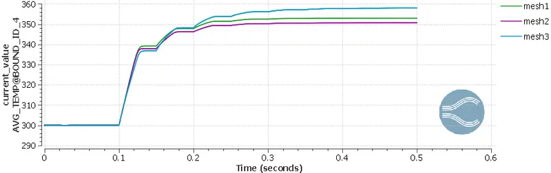
Outlet temperature for all the meshes in grid dependence study:

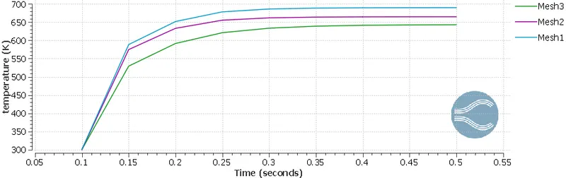
Output temperature of a point inside the solid region for all the meshes in grid dependence study:

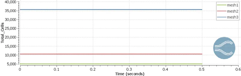
Number of cells in the grid dependence study

Effect of the supercycle interval on the output temperature inside the solid domain of Mesh 2

Observations and Conclusions:

From the above plots and contours we can make the following observations

1. In the current study, the outlet temperature for Mesh 1 and Mesh 2 are fairly converging and for Mesh3, since the y plus values are in the range of 10 and 30, the results obtained are in accurate
2. The increase in the number of cells for the grid dependence test is non-linear, hence care should be taken when deciding the grid dependence study
3. The Y plus values for the Mesh 1 and Mesh 2 are almost greater than 30 for the interface and hence the results obtained from these meshes are physically relevant
4. Reducing the super cycle interval length shows that the solid region reaches the steady state quite early which means that the time scale of the heat transfer in the solid region is relatively smaller
5. All cases reach to steady state temperature by 0.3 seconds and hence if we studying steady state phenomenon super cycle interval will not pose a problem.