Week-7 : Converting a detailed engine model to a FRM model

The objectives of the report are as follows:

1. To summarise the details of the tutorial-9 in GT-Suite for gaining a deeper understanding on Fast Running Model (FRM)
2. To use FRM builder to develop and simulate the parametric cases of turbocharged 6 cylinder diesel engine.

Section 1: Exploration of Tutorial-9 of GT-Suite

From the name of the concept, we understand that the simulation models build using this technique are for reducing the computational time requried. The major benefit of this simulation methodology is that it can quickly run different cases and provide a relatively accurate prediction. In contrast of the detailed models, where every part is modeled using a fine discretization, the FRM models try to fuse various parts of the physical system into a single part and use a coarse discretization. These changes lead to significant gains in computational speeds.

Since there is a trade-off between computational time and accuracy, the user must have sufficient knowledge to understand where they can implement a FRM or a detailed model. In general, FRM are built when we are testing the model using software or hardware in loop i.e. the simulation model might be connected with a real time ECU unit or a neural network model which instantaneously outputs certain values. If a detailed model is incorporated for this purpose, there will be significant delay because the simulation model will lag behind it physical counterparts.

In this section we will explore the tutorial number 9 offered by GT-Suite to understand how to build a FRM out of a detailed model.

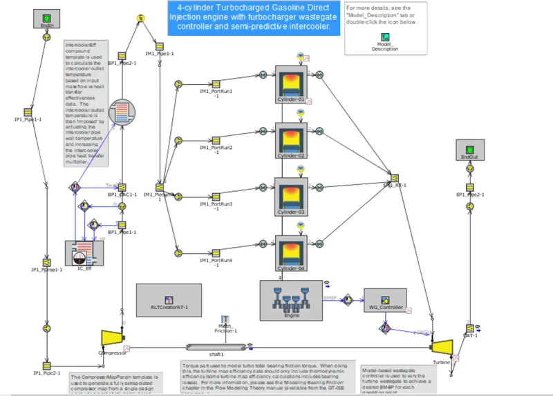
To begin, we observe the detailed model, which is the tutorial case by the name SI_4cyl_GDI_Turbo_WOT. The name indicates that the given detailed model is an engine with four cylinder, gasoline direct injection, is turbocharged and has a wastgate controller to manage the boosted pressure at the inlet. the image of the project map is as follows:

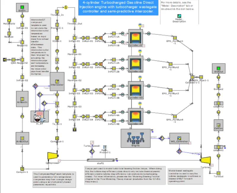
The objective of this tutorial is to simply the model based on accuracy and compare the engine performance parameters of the detailed model and the FRM. The GT-Suite showcases their feature of FRM converter for this problem, to help the user for gaining the knowledge of converting detailed model to a FRM.

Step 1: Exhaust Manifold

For this, FRM tagging is used from the Tools section. It provides us information for where to begin the simplification of the model. For instance, in this case, we begin with the exhaust manifold, since the gases in the that part are characterized with high velocities. These flow parameters greatly influence the Courant number and hence simplification of this part provides a great boost in terms of computational speed.

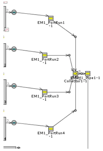
Step 2: Exhaust Pipe

Similar to the exhaust system, the exhaust pipes downstream of the turbine will be simplified.

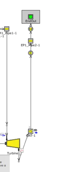
Step 3: Intake manifold

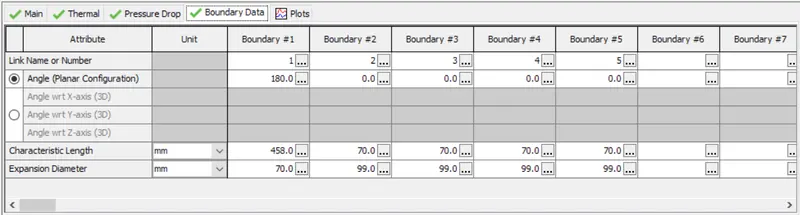
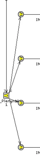
Similar to the previous parts, minor modifications are made to the characteristics length and expansion diameter attributes values of the combined flow

• Characteristic length is defined as the distance that fluid travels before crossing another boundary or impacting a surface.
• Since the flow can occur in any direction, backflow is a real possibility which can cause fluid backflow before impacting the plenum wall. Thus we provide characterisitic length of 70 mm.
• The expansion diameters for all other boundaries are equal to the plenum diameter multiplied by 1.4. This is also because of the backflow possibility, as the fluid will encounter a wider cross section.

Step 4: Compressor Outlet Pipe

Now, for the simplification of compressor outlet pipe, we use the simplify by accuracy option. The intercooler core has been replaced with a flowsplit and heat exchanger connection part.

Step 5: Intake pipes

Intake pipes are simplified for accuracy by using the FRM Convertor.

Step 6: Additional Changes

All the exhaust runner volumes are now merged into Single flow volume to find out the speed of the simulation.

Step 7: Cylinder Slaving

The final simplification to the model will utilize the Cylinder Slaving capability of the EngCylinder component. In this process, equations and wave-dynamics is solved for one master cylinder and other cylinder results are interpreted from the master cylinder instead of solving separately.

These changes along with all other simplifcations are shown in this figure

Section 2: Building FRM using FRM Builder approach

The following settings for the simulation is chose

• Bore = 102 mm
• Stroke = 115 mm
• CR = 17
• No of cylinder = 6
• Compression Ignition Engine,
• Twin Scroll Turbine
• GT Controller

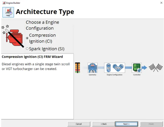
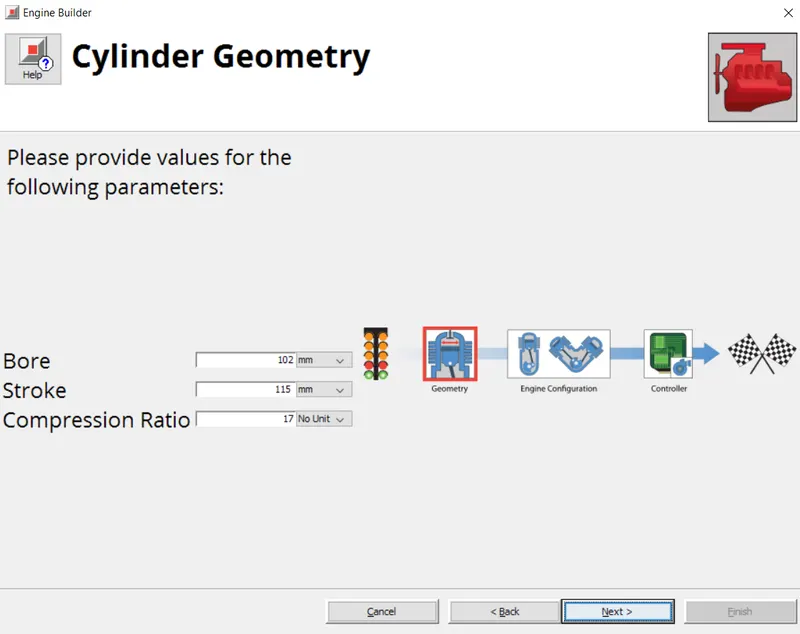
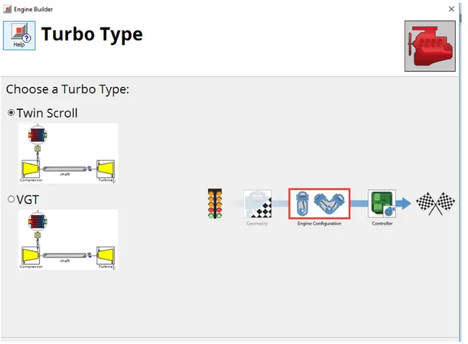
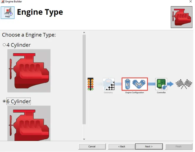
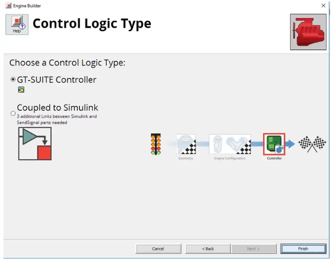
After selecting all the conditions as mentioned above, we finally show the FRM generated using the FRM Builder strategy

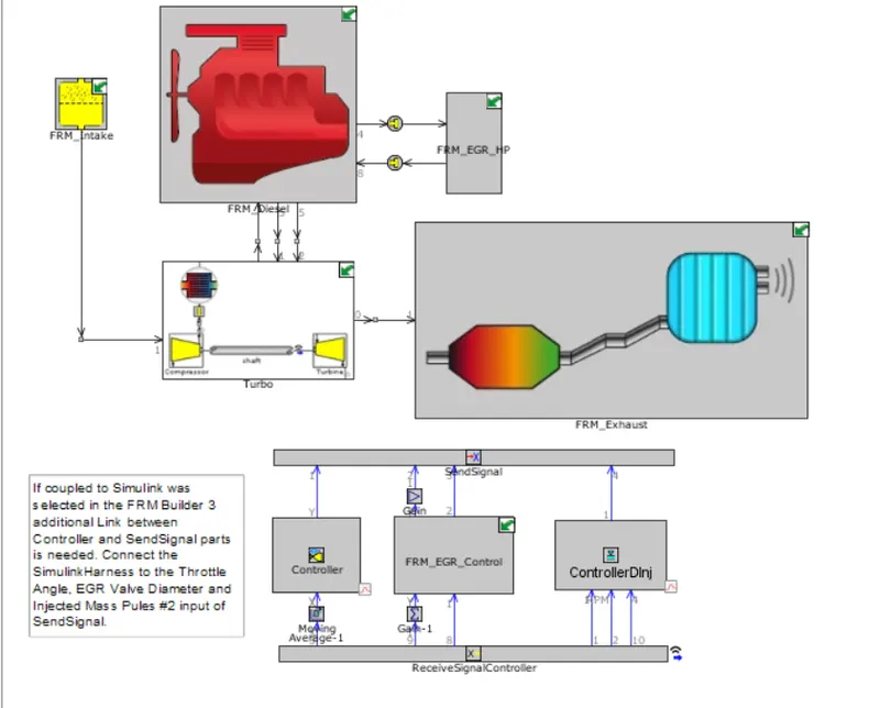
The result obtained from the FRM are as follows:

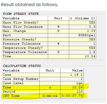
From the above results we can draw the following conclusions:

• If we directly compare the time taken to complete the simulation in detailed model as well as FRM it is seen that the detailed model took less time and FRM took more time, which is opposite of our expectation. But, if we look more closely, the more time taken by the FRM is because of number of periods for which the simulation ran.
  • FRM is run for 128 periods and time taken for same is 10.24 sec. But detailed model run for 75 periods and time taken for the same is 6 seconds, if the detailed model would have run for 128 periods the time taken would have been more than 10 seconds.

• Comparing the CPU time even after running 128 periods of simulation FRM took only 37.79 sec but the detailed model that run for 75 periods took 1:53:56, that is almost 2 hrs of cpu time. This is more than 1000x gains and make FRM very suitable for real-time systems.

• From the above result, we can conclude that for Sil, Hil and Mil type of simulations using FRM's will be a good option.