Week 5.1 - Mid term project - Solving the steady and unsteady 2D heat conduction problem

First, we design steady state solver for the two dimensional heat problem.

The structure of the main_s.m MATLAB file is explained as follows:

• The tolerance value is set as given, provide flags for different solver techniques like Jacobi, Gauss-Seidel and define `alpha` as the weighing factor for the Successive over-relaxation. Next, the space is discretized and boundary and initial conditions are applied as specified in the problem description.
• The steady_2D function file is called with different initial arguments to solve the 2D Heat conduction problem using Jacobi, Gauss-Seidel and SOR with Gauss Seidel methods

%%

clear 
close all
clc

%% Setting the initial values

tol = 1e-4;
alpha = 1;
alpha_best = 1.6;
iter_scheme_jac = 1;
iter_scheme_gs = 2;

dx = 0.1; % Space discretization in x dir
dy = 0.1; % Space discretization in y dir
x = 0:dx:1;
y = 0:dy:1;
nx = size(x,2);  % No. of nodes in x dir
ny = size(y,2);  % No. of nodes in y dir
[X,Y] = meshgrid(x,y);

T = 400*ones(11,11);    % Domain
T(1,:) = 600;   % Top Boundary
T(:,end) = 800;   % Right Boundary
T(end,:) = 900;   % Bottom Boundary

T(1,1) = (T(1,2) + T(2,1))/2;   % Top Left
T(1,end) = (T(1,end-1) + T(2,end))/2;   % Top Right
T(end,end) = (T(end,end-1) + T(end-1,end))/2;   % Bottom Right
T(end,1) = (T(end,2) + T(end-1,1))/2;   %Bottom Left

%% Calling the function for Jacobi

[T_final_jac,n_iter] = steady_2D(T,nx,ny,dx,dy,iter_scheme_jac,tol,alpha,X,Y,1);

disp(n_iter)

%% Calling the function for Gauss-Seidel

[T_final_gs,n_iter_new] = steady_2D(T,nx,ny,dx,dy,iter_scheme_gs,tol,alpha,X,Y,2);

disp(n_iter_new)

%% Calling the function with SOR 


[T_final_accel_s,n_iter_new] = steady_2D(T,nx,ny,dx,dy,iter_scheme_gs,tol,alpha_best,X,Y,3);

disp(n_iter_new)

The steady_2D.m MATLAB function is designed to be a generalized solver for simulating the steady 2D heat conduction, and returning the final temperature field and number of iterations required. The structure of the steady_2D.m MATLAB File is as follows:

• The definitions for Jacobi and Gauss-Seidel are implemented and the solver chooses a specific technique based on the flag 'iter_scheme' provided to it
• Some important temporary variables are set up which makes the implementation of the solver cleaner and 2 copies of the initial temperature field are assigned to 'T' and 'T_old'
• The main loop is a 'while' loop which is runs till the error (the error is defined as the absolute maximum temperature deviation in the entire domain) is larger than the specified tolerance
  • The inner two 'for' loops calculates the new temperature for each discrete point in the domain depending on the iterative solver chosen by the user
  • The temperature is updated in SOR format, so if the user would like to use standard Jacobi or Gauss-Seidel Methods, then the alpha has to be set as 1
• The updated temperature field for each iteration is plotted with appropriate labels and colourbar is plotted using the contour_2D_plot function

function [T,n_iter] = steady_2D(T_initial,nx,ny,dx,dy,iter_scheme,tol,alpha,X,Y,fig_num)
    %% Jacobi = 1 and Gauss-Seidel = 2

    if iter_scheme == 1
        T_h = @(iter_x,iter_y,T,T_old) T_old(iter_x-1,iter_y) + ...
                                       T_old(iter_x+1,iter_y);
        T_v = @(iter_x,iter_y,T,T_old) T_old(iter_x,iter_y-1) + ...
                                       T_old(iter_x,iter_y+1);
    elseif iter_scheme == 2
        T_h = @(iter_x,iter_y,T,T_old) T(iter_x-1,iter_y) + ...
                                       T_old(iter_x+1,iter_y);
        T_v = @(iter_x,iter_y,T,T_old) T(iter_x,iter_y-1) + ...
                                       T_old(iter_x,iter_y+1);
    end

    %% Setting up

    K = 2*(dx^2 + dy^2)/(dx^2*dy^2);
    T = T_initial;
    T_old = T_initial;
    error = 1e10;
    n_iter = 1;

    %% Main loop

    while (error > tol)

        for i=2:nx-1
            for j=2:ny-1
            
            T_update_h = (1/(K*dx^2))*(T_h(i,j,T,T_old));
            T_update_v = (1/(K*dy^2))*(T_v(i,j,T,T_old));
            T_update = T_update_h + T_update_v;
            T(i,j) = (1-alpha)*T_old(i,j) + alpha*(T_update);

            end
        end

        error = max(max(abs(T-T_old)));
        T_old = T;
        n_iter = n_iter + 1;

        contour_2D_plot(X,Y,T,fig_num)

    end

The detailed colour map of the temperature field of the 2D domain is plotted by the contour_2D_plot function. The structure of the contour_2D_plot.m MATLAB file is as follows

• Using the meshgrid and temperature values, plot the temperature field using the contourf function
• Provide information about the contour by providing labels and colormap

function contour_2D_plot(X,Y,T,fig_num)

    figure(fig_num)
    [c,h] = contourf(X,Y,T); 
    colormap jet
    clabel(c,h)
    colorbar 
    set(gca,'YDir','reverse')
    xlabel('X-direction')
    ylabel('Y-direction')
    title('Temperature distribution (in K) on the 2D domain');

    pause(0.03) 

end

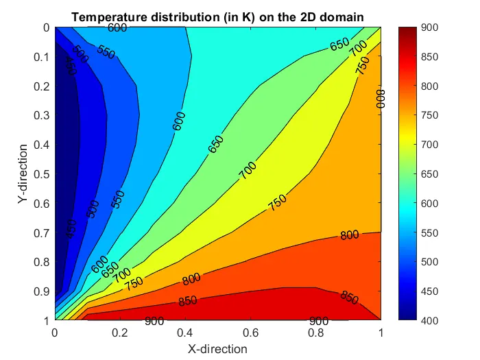
The temperature field and the number of iterations for each iterative solver are provided and we summarize the conclusions for the same

• Jacobi Method

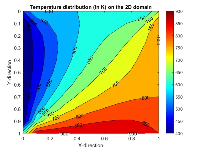
• Gauss-Seidel Method

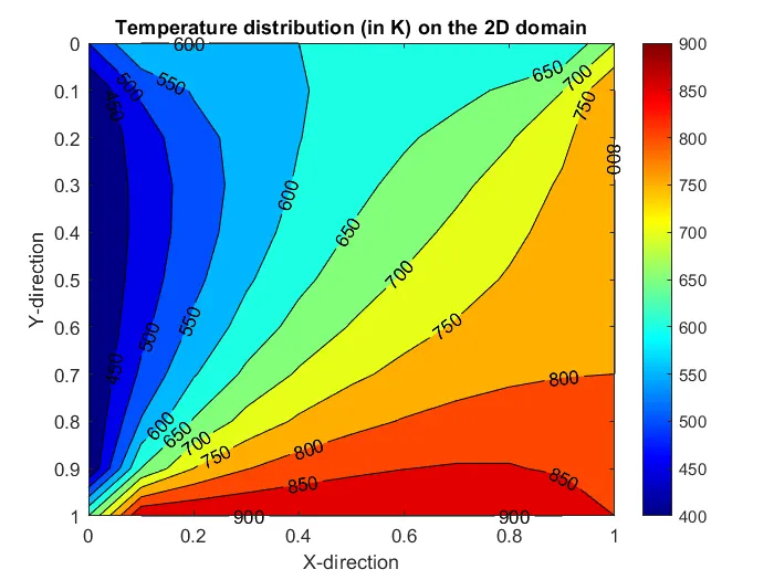
• SOR

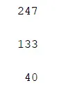
• The number of iterations required for Jacobi, Gauss-Seidel and SOR

The observations and conclusions for the steady state solver are as follows:

1. All the three methods provide virtually identical solutions as per the provided solutions. We can conclude that the solver code has been implemented correctly
2. The number of iterations required for Jacobi method are the highest followed by the Gauss-Seidel (~50% reduction) and the least amount are taken by the SOR method (~80% reduction)
3. The relaxtion factor `alpha` which provides the most reductions was found out to be 1.6 (values between 1.1 and 1.6 also improve the performance of the solver) for the current initial conditions

To solve the unsteady 2D heat conduction problem, we implement two transient solvers: 1) Explicit Solver 2) Implicit Solver. The simulation of the unsteady heat flow problem is implemented in the main_t.m MATLAB file.

The structure of the main_t.m MATLAB file is as follows

• Similar to the steady state solver, we provide the conditons for the simualtion and initial and the boundary values for the discretized domain.
  • The `alpha` here signifies the heat diffusivity coefficient while the `omega` represents the relaxtion factor
  • We consider time-stepping along with the discretization of the space (CFL criteria should be met for explicit solver)
• The different implicit iterative solvers are instantiated using the same transient_2D_im MATLAB function
• The explicit solver is instantiated by using the transient_2D_ex MATLAB function

%%

clear 
close all
clc

%% Setting the initial values

% Setting solver settings
tol = 1e-4;
omega = 1;
omega_best = 1.2;
iter_scheme_jac = 1;
iter_scheme_gs = 2;

% Time Discretization
dt = 0.002;     % Based from explicit schemes 0.002 < 0.25*0.1^2/1.1
nt = 200;

% Domain Discretization
dx = 0.1; % Space discretization in x dir
dy = 0.1; % Space discretization in y dir

x = 0:dx:1;
y = 0:dy:1;
nx = size(x,2);  % No. of nodes in x dir
ny = size(y,2);  % No. of nodes in y dir
[X,Y] = meshgrid(x,y);

% Thermal Properties

alpha = 1.1; % Based from explicit schemes < 0.25*0.1^2/1.1

T = 400*ones(11,11);    % Domain
T(1,:) = 600;   % Top Boundary
T(:,end) = 800;   % Right Boundary
T(end,:) = 900;   % Bottom Boundary

T(1,1) = (T(1,2) + T(2,1))/2;   % Top Left
T(1,end) = (T(1,end-1) + T(2,end))/2;   % Top Right
T(end,end) = (T(end,end-1) + T(end-1,end))/2;   % Bottom Right
T(end,1) = (T(end,2) + T(end-1,1))/2;   %Bottom Left


%% Calling the function for Jacobi

[T_final_jac] = transient_2D_im(T,nx,ny,nt,dx,dy,dt,iter_scheme_jac,tol,alpha...
                                 ,omega,X,Y,1);

%% Calling the function for Gauss-Seidel

[T_final_gs] = transient_2D_im(T,nx,ny,nt,dx,dy,dt,iter_scheme_gs,tol,alpha...
                                      ,omega,X,Y,2);

%% Calling the function with SOR 
 
[T_final_accel] = transient_2D_im(T,nx,ny,nt,dx,dy,dt,iter_scheme_gs,tol,alpha...
                                  ,omega_best,X,Y,3);

%% Explicit Scheme

[T_exp_sol] = transient_2D_ex(T,nx,ny,nt,dx,dy,dt,tol,alpha,...
                               X,Y,4);

The transient solver transient_2D_im is a generalized solver which can simulate different iterative schemes. The structure of the transient_2D_im.m MATLAB file is as follows

• The definitions of the Jacobi and Gauss-Seidel Method have been implemented and can be selected by providing the appropriate flag
• Temporary variables are set up, and three copies of the initial temperature field are made
• The algorithm consists of 4 loops
  • The first 'for' loop is for stepping in time. 'T' denotes the temperature field at current time step while 'T_prev' represents the temperature field of the previous time step
  • The second 'while' loop is for convergence of the temperature field at the next time step using the iterative solver technique chosen. 'T_old' signifies the temperature field values till it is converged for a given time step
  • The inner two 'for' loops are for updating the temperature values in the discretized domain
• The contour at each time step is plotted using the contour_2D_plot which is explained in the steady solvers

function [T] = transient_2D_im(T_initial,nx,ny,nt,dx,dy,dt,iter_scheme,tol,alpha...
                                  ,omega,X,Y,fig_num)
    %% Jacobi = 1 and Gauss-Seidel = 2

    if iter_scheme == 1
        T_h = @(iter_x,iter_y,T,T_old,K1) K1*T_old(iter_x-1,iter_y) + ...
                                          K1*T_old(iter_x+1,iter_y);
        T_v = @(iter_x,iter_y,T,T_old,K2) K2*T_old(iter_x,iter_y-1) + ...
                                          K2*T_old(iter_x,iter_y+1);
    elseif iter_scheme == 2
        T_h = @(iter_x,iter_y,T,T_old,K1) K1*T(iter_x-1,iter_y) + ...
                                          K1*T_old(iter_x+1,iter_y);
        T_v = @(iter_x,iter_y,T,T_old,K2) K2*T(iter_x,iter_y-1) + ...
                                          K2*T_old(iter_x,iter_y+1);
    end

    %% Setting Up

    K1 = alpha*dt/dx^2;
    K2 = alpha*dt/dy^2;
    K = 1 + 2*K1 + 2*K2;
    T = T_initial;
    T_prev = T_initial;
    T_old = T_initial;

    %% Main loop

    for i=1:nt

        error = 1e10;

        while error > tol
            for j=2:nx-1
                for k=2:ny-1

                T_update_h = (1/K)*(T_h(j,k,T,T_old,K1));
                T_update_v = (1/K)*(T_v(j,k,T,T_old,K2));
                T_update = T_prev(j,k)/K + T_update_h + T_update_v;
                T(j,k) = (1-omega)*T_old(j,k) + omega*(T_update);
                   
                end
            end

            error = max(max(abs(T-T_old)));
            T_old = T;

        end

        T_prev = T;
        contour_2D_plot(X,Y,T,fig_num)

    end
    
end

The explicit transient solver is implemeted in the transient_2D_ex MATLAB function. The structure for the transient_2D_ex.m MATLAB file is as follows

• Setting up temporary variables and anonymous functions to simply the implementation of the explicit formula
• The main algorithm has three loops
  • The first 'while' loop is for stepping in time and measuring the error difference between the current and previous time step values as stopping criteria (The relative error criteria is only suitable for problems which have steady state solution, which is the case in the current problem)
  • The two 'for' loops are for updating the temperature values for the next time step
• Time step counter is updated and the the temperature field is plotted using the contour_2D_plot.m function

function [T] = transient_2D_ex(T_initial,nx,ny,nt,dx,dy,dt,tol,alpha,...
                               X,Y,fig_num)
    %% Setting Up

    K1 = alpha*dt/dx^2;
    K2 = alpha*dt/dy^2;
    K = 1 - 2*K1 - 2*K2;
    T = T_initial;
    T_prev = T_initial;
    T_h = @(iter_x,iter_y,T_old,K1) K1*T_old(iter_x-1,iter_y) + ...
                                          K1*T_old(iter_x+1,iter_y);
    T_v = @(iter_x,iter_y,T_old,K2) K2*T_old(iter_x,iter_y-1) + ...
                                          K2*T_old(iter_x,iter_y+1);
    niter = 1;
    error = 1e10;
     
    %% Main Loop

    while(niter <= nt && error > tol)

        for j=2:nx-1
            for k=2:ny-1

                T(j,k) = K*T_prev(j,k) + T_h(j,k,T_prev,K1) + T_v(j,k,T_prev,K2);

            end 
        end

        error=max(max(abs(T-T_prev)));
        T_prev = T;
        niter=niter + 1;
        contour_2D_plot(X,Y,T,fig_num)

    end

end

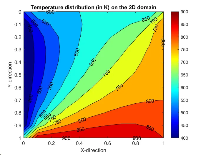
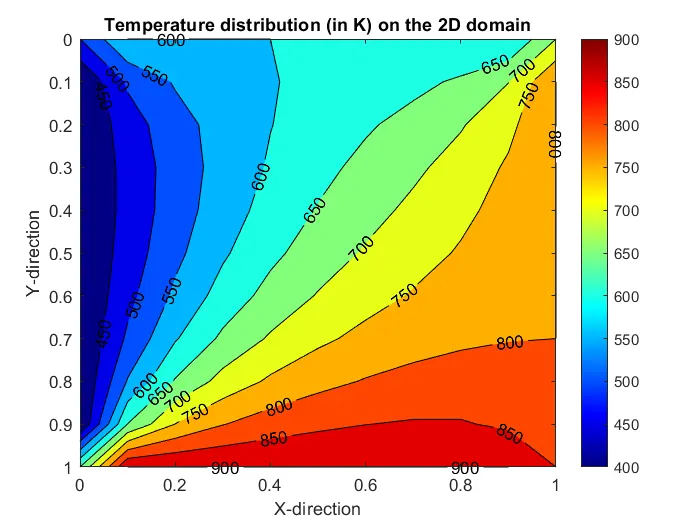
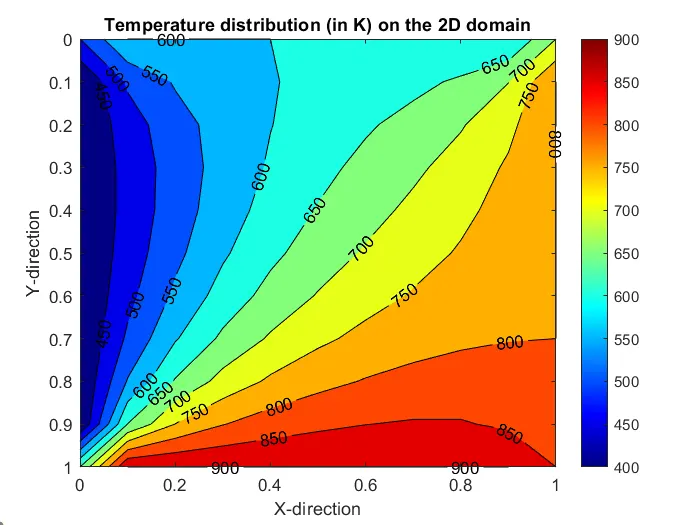
The contours, results and conclusions obtained form the transient solvers are as follows

• Jacobi Method

• Gauss-Seidel Method

• SOR Method

• Explicit Method

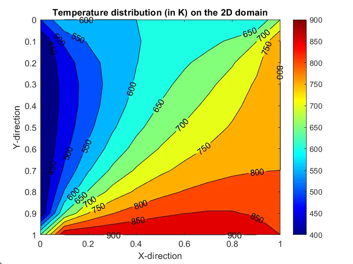
The results and conclusions for the transient solver for 2D unsteady heat conduction is as follows:

1. The results for all 4 methods are virtually identical. This concludes that the implementation of the transient scheme has been done correctly
2. We observe that `alpha = 1.1`, the explicit solver requires a time step smaller 0.0023 for stability because of the CFL criteria but the implicit solvers can run on larger time steps and thus can provide accurate solutions in smaller amount of computation time
3. By calculating the norm distance between steady state results and the transient schemes, we find the SOR with appropriate over-relaxation factor provides the most accurate solutions