Week 3.5 - Deriving 4th order approximation of a 2nd order derivative using Taylor Table method
- From the formula provided for determing the order of accuracy for central schemes, we can conclude that the size of the numerical stencil for the 4th order accurate central difference scheme for 2nd derivative is 5.
- The finite difference representation for the aformentioned scheme is as follows and let:
`{partial^2 f}/{partial x^2} = af_{i-2} + bf_{i-1} + cf_{i} + df_{i+1} + ef_{i+2} + O(Delta x^4 )`
- The Taylor Table method for the given problem is as shown below
| `f_{i}` | `f'_{i}` | `f''_{i-2}` | `f'''_{i-2}` | `f''''_{i-2}` | |
| `f_{i-2}` | `1` | `{-2 Deltax}/{1!}` | `{4 Deltax^2}/{2!}` | `{-8 Deltax^3}/{3!}` | `{16 Deltax^4}/{4!}` |
| `f_{i-1}` | `1` | `{- Deltax}/{1!}` | `{ Deltax^2}/{2!}` | `{- Deltax^3}/{3!}` | `{ Deltax^4}/{4!}` |
| `f_{i}` | `1` | `0` | `0` | `0` | `0` |
| `f_{i+1}` | `1` | `{Deltax}/{1!}` | `{ Deltax^2}/{2!}` | `{ Deltax^3}/{3!}` | `{ Deltax^4}/{4!}` |
| `f_{i+2}` | `1` | `{2 Deltax}/{1!}` | `{4 Deltax^2}/{2!}` | `{8 Deltax^3}/{3!}` | `{16 Deltax^4}/{4!}` |
- Substituting the coefficients of the Talyor Table coefficients in the finite difference formula and comparing the LHS and RHS of the equation we get a system of linear equations for the variables `a,b,c,d,e`
- These system of equations are solved using MATLAB function taylor_central.m as shown below
function X = taylor_central() A = [1 -2/factorial(1) 4/factorial(2) -8/factorial(3) 16/factorial(4); ... 1 -1/factorial(1) 1/factorial(2) -1/factorial(3) 1/factorial(4); ... 1 0 0 0 0; ... 1 1/factorial(1) 1/factorial(2) 1/factorial(3) 1/factorial(4); ... 1 2/factorial(1) 4/factorial(2) 8/factorial(3) 16/factorial(4)]; A = A.'; b = [0; 0; 1; 0; 0]; X = A\b; end - The values for the variables are as follows:
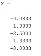
- These system of equations are solved using MATLAB function taylor_central.m as shown below
- Similarly, using the order of accuracy formula for the skewed schemes, we obtain that for 4th order forward/backward scheme for second derivative the size of the numerical stencil is 6
- Finte difference representation for the backward scheme is as follows
`{partial^2 f}/{partial x^2} = af_{i-5} + bf_{i-4} + cf_{i-3} + df_{i-2} + ef_{i-1} + gf_{i} + O(Delta x^4 )`
- Finte difference representation for the forward scheme is as follows
`{partial^2 f}/{partial x^2} = af_{i} + bf_{i+1} + cf_{i+2} + df_{i+3} + ef_{i+4} + gf_{i+5} + O(Delta x^4 )`
- Using similar technqiue for the forward and backward schemes as implemented for the central scheme, we make the Taylor table, substitute it in the finite difference representation formula and derive the system of equations for the variables `a,b,c,d,e,g`
- The system of equations are solved by the MATLAB functions taylor_forward and taylor_backward and the value of the variables are obtained as follows
- Forward Difference Scheme
function X = taylor_forward() A = [1 0 0 0 0 0; ... 1 1/factorial(1) 1/factorial(2) 1/factorial(3) 1/factorial(4) 1/factorial(5); ... 1 2/factorial(1) 4/factorial(2) 8/factorial(3) 16/factorial(4) 32/factorial(5);... 1 3/factorial(1) 9/factorial(2) 27/factorial(3) 81/factorial(4) 243/factorial(5); ... 1 4/factorial(1) 16/factorial(2) 64/factorial(3) 256/factorial(4) 1024/factorial(5);... 1 5/factorial(1) 25/factorial(2) 125/factorial(3) 625/factorial(4) 3125/factorial(5)]; b = [0; 0; 1; 0; 0; 0]; A = A.'; X = A\b; end - The value of the variables is as follows
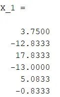
- Backward Difference Scheme
function X = taylor_backward() A = [1 -5/factorial(1) 25/factorial(2) -125/factorial(3) 625/factorial(4) -3125/factorial(5); ... 1 -4/factorial(1) 16/factorial(2) -64/factorial(3) 256/factorial(4) -1024/factorial(5); ... 1 -3/factorial(1) 9/factorial(2) -27/factorial(3) 81/factorial(4) -243/factorial(5); ... 1 -2/factorial(1) 4/factorial(2) -8/factorial(3) 16/factorial(4) -32/factorial(5);... 1 -1/factorial(1) 1/factorial(2) -1/factorial(3) 1/factorial(4) -1/factorial(5); ... 1 0 0 0 0 0]; A = A.'; b = [0; 0; 1; 0; 0; 0]; X = A\b; end - The value of the variables for this scheme are as follows
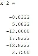
- Forward Difference Scheme
To compare the performance of the three numerical schemes, we compare the difference between the analytical and the numerical approximation of the second derivative of the function `f(x) = e^x.cos(x)` at x=1 for the dx=[`10^{-2};10^{-1};10`]
We devise the main.m file to plot the error with respect to dx for the three schemes. The main sections of the code are explained as follows:
- We define the given data and function and also calculate the analytical second derivative and store it in the variable 'analytic'
- We calculate the coefficients for the central, forward and backward schemes from the functions defined above and use them to numerically calculate the second derivative
- We calculate the absolute error and plot the Error with respect to dx on loglog graph with appropriate legend and labels
- We calculate the slope of the graphs to verify the order of accuracy for the schemes using polyfit
%% clear close all clc %% Initial Data f = @(x) exp(x).*cos(x); x = 1*ones(1,20); dx = linspace(1e-2,1e-1,20); %% Analytic Derivative df = @(x) -2.*exp(x).*sin(x); analytic = df(x); %% Taylor Table X = taylor_central(); % Central Difference X_1 = taylor_forward(); % Skewed Right X_2 = taylor_backward(); % Skewed Left %% Taylor schemes applied Y = taylor_central_app(f,X,x,dx); Y_1 = taylor_forward_app(f,X_1,x,dx); Y_2 = taylor_backward_app(f,X_2,x,dx); %% Error cal and plotting E = abs(Y - analytic); E_1 = abs(Y_1 - analytic); E_2 = abs(Y_2 - analytic); loglog(dx,E,'-o'); hold on; loglog(dx,E_1,'-x'); loglog(dx,E_2,'-*'); legend('central','forward','backward','Location','best') P = polyfit(log(dx),log(E),1); P_1 = polyfit(log(dx),log(E_1),1); P_2 = polyfit(log(dx(:,1:end-8)),log(E_2(:,1:end-8)),1); slope = P(1); slope_1 = P_1(1); slope_2 = P_2(1);
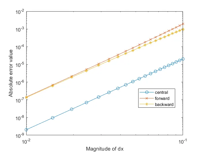
From the graph, we note the following observations:
- The slopes for the central, forward and backward schemes using the polyfit function are 3.9999, 4.1284 and 3.8956 respectively. Hence, this is suitable verification for the correctness of our schemes
- The size of stencil of central scheme is smaller than that of the forward and backward schemes eventhough the order of accuracy are same. We can conclude that central schemes are computationally more efficient.
- We observe that the central schemes cannot be used at the boundaries due to the absence of points on the boundary side. This is were we can use the skewed schemes to our advantage for getting accurate results.