Week 9 - Mini project - Flow over an Airfoil

Aim:

To setup simulation over NACA 2412 airfoil and to carry out a systematic study of the effect of angle of attack and turbulence models on the drag and lift coefficients.

Objectives:

1. Provide a brief introduction on airfoil theory and provide formulaes for the quntification of lift and drag coefficients.
2. Setup the geometry of varying angles of attack (1, 5, 10, 15) by enclosing the geometry in a boundaing box for external aerodynamic simulation.
3. Setup the case for the simulations with appropriate mesh settings and turbulence models
4. Discuss the results and provide conclusions on the systematic study.

Theory:

The aerofoils are structures which have a special geometrical body that generates mechanical forces when there is a relative motion between it and the fluid in which it is immersed. A simplistic aerofoil profile in action can be depicted as follows:

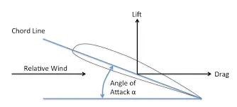
In this figure the chord line joins the leading and trailing edges and the upper and lower surfaces are joined by a line which is perpendicular to the chord line. The angle of attack (α) is defined as the angle between the vector of the velocity and the chord line of the aerofoil. These geometric parameters play an important role in determining the aerodynamic performance of the aerofoil in the form of the lift and drag forces and the pitching moment.

The pressure forces are higher on the lower surface and it is called the “pressure” side of the aerofoil while on the top surface the fluid accelerates and has a lower pressure. Hence, this surface is termed as the “suction” side of the aerofoil. The pressure differences on the surfaces give rise to the forces which act on the aerofoil. The lift force is defined as the force acting perpendicular to the incoming airflow while the force acting parallel to the airflow is termed as the drag force.

To compare the performance of different aerofoil profiles, the forces defined above are non-dimensionalized. The non-dimensional equivalents for the forces are lift coefficient and drag coefficient. They are defined as follows:

● Lift coefficient is defined as the ratio of the lift force generated due to the pressure differences on the top and bottom surfaces of the aerofoil and the dynamic force of the fluid. Mathematically, it can be represented by the following equation

`C_L = F_L/{0.5 times rho times v^2 times A}`

● Drag coefficient is defined as the ratio drag force generated due to sum the pressure difference between the leading and trailing edges and the friction forces acting on the aerofoil surface due to the viscous nature of the fluid and the dynamic force of the fluid. Mathematically, it can be represented by the following equation

`C_D = F_D/{0.5 times rho times v^2 times A}`

In this study, we will study the effects of the geometrical factors example angle of attack (α) and turbulence models on the lift and drag forces for Reynolds Number of the flow as 200000.

Geometry:

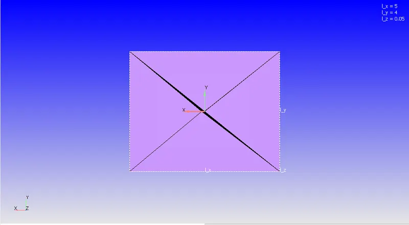
The airfoil geometry is generated using the .dat file from the website known as Airfoil Tools. After plotting the points on the surface of the airfoil geometry, it is patched to make it a solid body. This patched body is enclosed by a rectangular domain to simulate the effects of airfoil placed in the wind tunnel. From the literature it is known that the streamwise length of the domain should be kept 50 times the chord length and the lateral length should be kept 30 times the chord length.

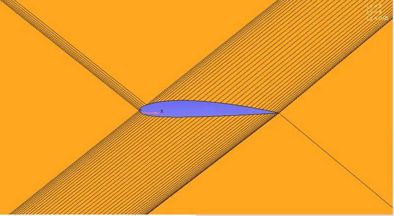
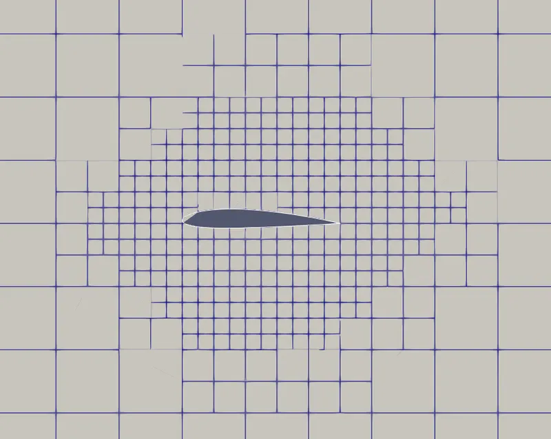
The airfoil geometry is subtracted from the enclosed volume to simulate the flow problem. The computational domain and its closeup is shown in the following figure:

Computational Domain:

Closeup to visualize the airfoil:

Case Setup:

The case setup for the current study is carried out using the CONVERGE Studio Case Setup GUI. The following settings have been chosen for the simulation in the respective subtree

• Application subtree:
  • Due to the relatively simple nature of the model, the Time based application was selected
• Materials subtree:
  • Predefined mixture of standard air with gas simulation default settings was used.
  • The global transport parameters were set to default values
  • The standard air consists of oxygen and nitrogen species which are assumed to be non-reacting mixtures.
• Simulation parameters subtree:
  • Fully compressible transient simulation with full hydrodynamic capacity is used for the simulation.
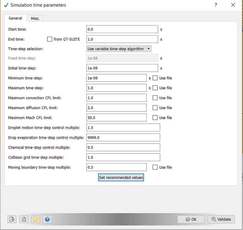
  • Using the inlet velocity of 30.14 m/s (calculated from the Re = 200000) and the streamwise length of the domain of 5 m, we can calculated the flow through time as 0.166. For achieving fully developed conditions, we decide the end time of the simulation as 0.2 second.
  • The initial time step is set to 1e-9 which is also the minimum time step for the simulation. The maximum time step is set to 1 second. The CFL criteria for the convection is set to 1 and for diffusion is set as 2. The variable time-step algorithm is used for the time stepping in the problem.

• A standard density based PISO algorithm was chosen as the Navier-Stokes equation solver with default settings

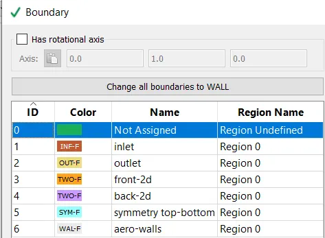
• Boundary Conditions subtree:
  • Inlet: Pressure = Zero Normal Gradient , Velocity = 30.14 m/s in the x-direction, Temperature = Fixed value of 300K, Species = Standard Air, Turbulent kinetic energy and turbulent dissipation = default values
  • Outlet: Pressure = Static pressure of 101325 Pa (1 bar), Velocity = Zero Normal Gradient, Temperature = Backflow value of 300K, Species = Backflow value of Standard Air, Turbulent kinetic energy and turbulent dissipation = default values
  • Airfoil Wall: Pressure = zero normal gradient, Velocity = Law of the Wall (stationary), Temperature = Law of the wall with wall temperature as 300K, Turbulent kinetic energy = zero normal gradient and Turbulent dissipation = Wall model
  • Top and Bottom walls: Symmetry.
  • Front and Back walls: Two dimensional conditions

• Initial Conditions subtree:
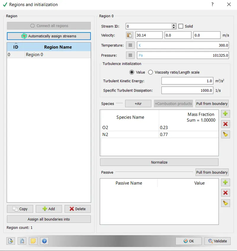
  • Fluid domain is initialized by filling it standard Air with velocity equal to inlet velocity, temperature of 300K and pressure set at 101325 Pa.

• Physical Models subtree:
  
  • For the current simulation, either RNG k-`epsilon` or k-`omega` SST turbulence models are used to quantify their effects on the calculation of lift and drag coeffficients.
• Grid Control subtree:
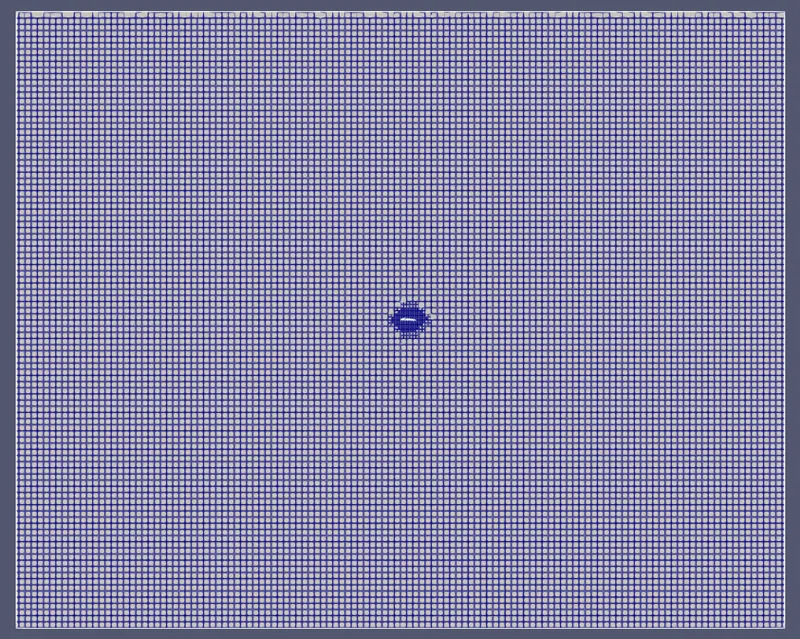
  • The base grid settings for cell dimension is set to 0.04m in all directions.
  • A fixed embedding is provided on the airfoil walls which is permanent. The scale is set to 2 and the embedding layers is set to 6.
• Output subtree:
  • To calculate the forces in the principal directions on the airfoil, we switch on the wall output to boundaries only.

Simulation Results:

The results of the systematic study for the different angles of attack (1, 5, 10, 15) and effects of the turbulence models have been summarized in this section.

Finally, we conclude this section by, plotting the variation of the lift and drag coefficients with the angles of attack.

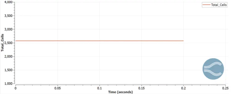
Cell Count:

Variation of the Drag force with time for angle of attack = 1 and Turbulence Model: k-`omega` SST

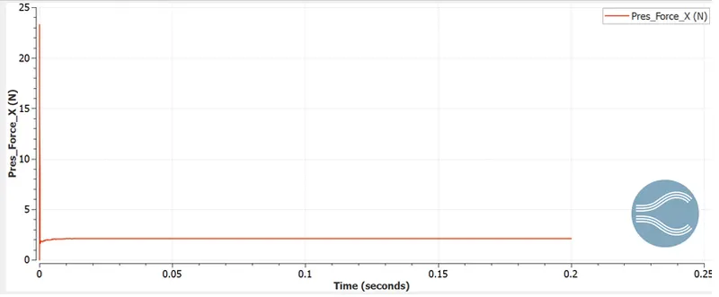
Variation of the Drag force with time for angle of attack = 1 and Turbulence Model: RNG k-`epsilon`

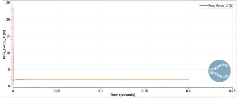
Variation of the Drag force with time for angle of attack = 5 and Turbulence Model: k-`omega` SST

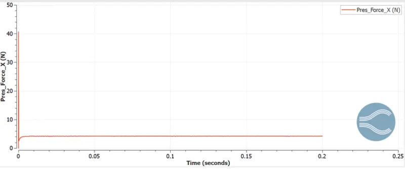
Variation of the Drag force with time for angle of attack = 5 and Turbulence Model: RNG k-`epsilon`

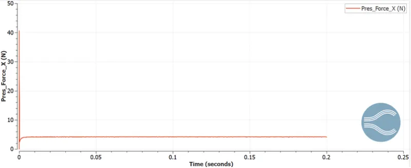
Variation of the Drag force with time for angle of attack = 10 and Turbulence Model: k-`omega` SST

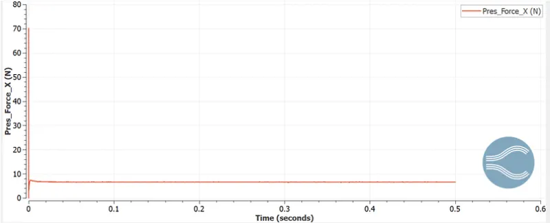
Variation of the Drag force with time for angle of attack = 10 and Turbulence Model: RNG k-`epsilon`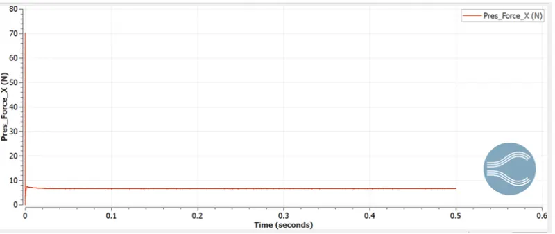

Variation of the Drag force with time for angle of attack = 15 and Turbulence Model: k-`omega` SST

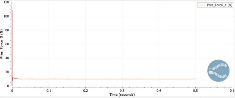
Variation of the Drag force with time for angle of attack = 15 and Turbulence Model: RNG k-`epsilon`

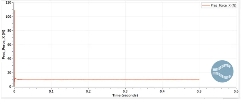
Variation of the Lift force with time for angle of attack = 1 and 5 and Turbulence Model: k-`omega` SST

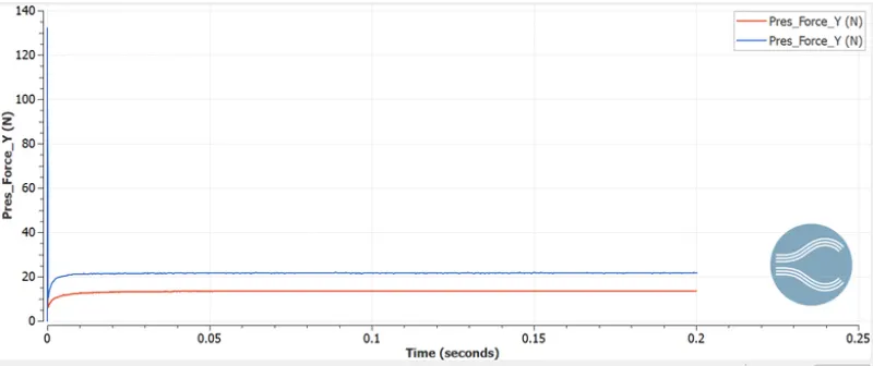
Variation of the Lift force with time for angle of attack = 1 and 5 and Turbulence Model: RNG k-`epsilon

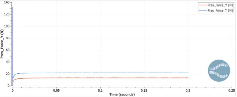
Variation of the Lift force with time for angle of attack = 10 and 15 and Turbulence Model: k-`omega` SST

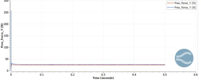
Variation of the Lift force with time for angle of attack = 10 and 15 and Turbulence Model: RNG k-`epsilon

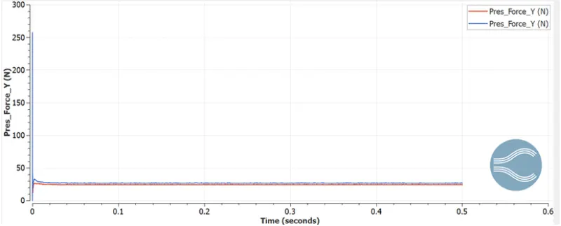
The principal forces in the x and y directions are converted into the lift and drag coefficients by using the fomulaes mentioned in the theory sections and using the frontal area as the chord length of the domain. These calculations are tabulated in the following table

Angle of attack	Turbulence Model	Drag Force	Lift Force	Drag Coefficient	Lift Coefficient
1	k-`omega` SST	2.11393	13.3786	0.0386	0.2431
1	RNG k-`epsilon`	2.11429	13.3234	0.0300	0.2448
5	k-`omega` SST	4.21886	21.5473	0.077	0.3900
5	RNG k-`epsilon`	4.18531	21.5517	0.076	0.3939
10	k-`omega` SST	6.55044	24.4601	0.1298	0.4801
10	RNG k-`epsilon`	6.59676	24.5970	0.1200	0.4800
15	k-`omega` SST	9.91812	19.8199	0.1878	0.3901
15	RNG k-`epsilon`	9.80275	19.6801	0.1865	0.3976

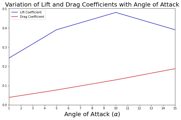
Variation of the drag and lift coefficients with angles of attack for the k-`omega` SST model

Variation of the yplus for all angles of attack with time

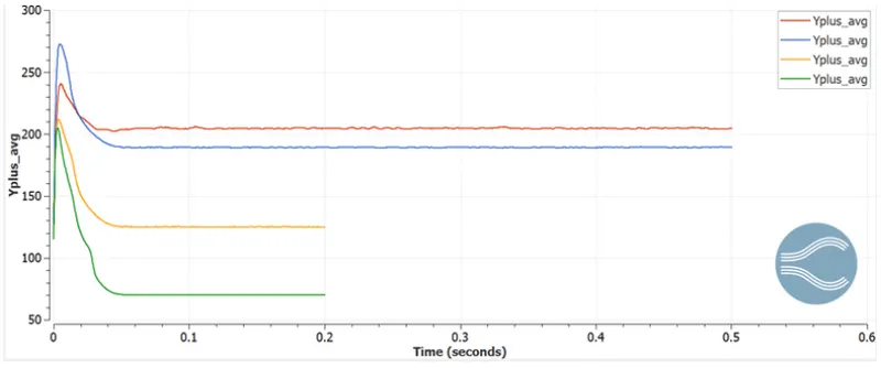
Although the average y plus value increases with the increase in angle of attack but the y+ is between 30 and 300 hence the turbulence models are valid for the current simulations.

Mesh with boundary embedding on the airfoil

Mesh Closeup

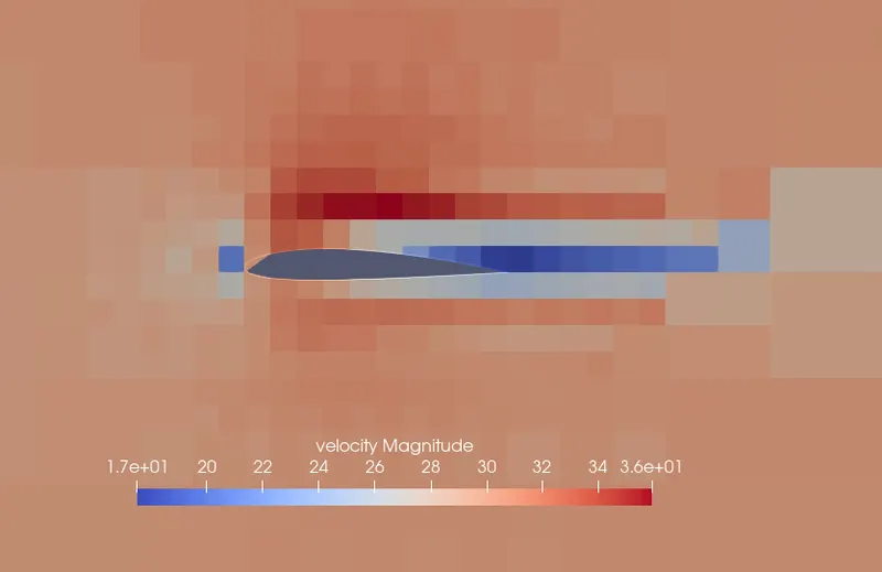
Velocity Contour

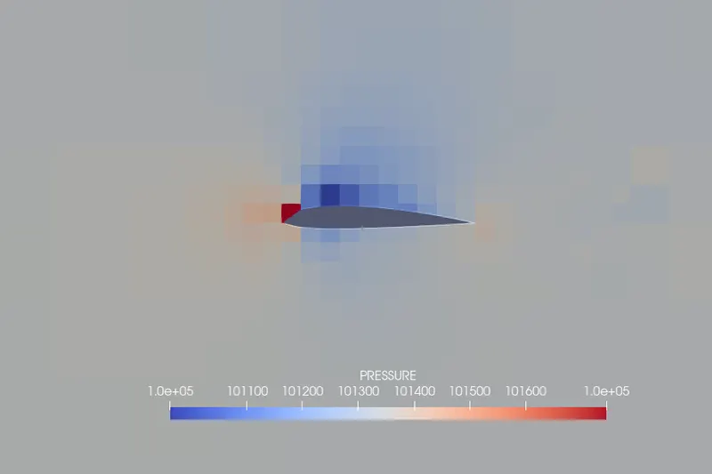
Pressure Contour

Animation:

Flow Velocity development with time animation: Animation Link

Conclusions:

From the above figures we can draw the following conclusions

1. The lift and drag coefficient becomes sufficiently constant at the completion of the simulations. This means that the calculations of the lift and drag coefficient have proper physical interpretation.
2. The Lift increases till angle of attack 10 and then decreases. This trend is corresponding to the experimental observations.
3. The Drag coefficient keeps on increasing with the angle of attack. This is expected as the airfoil geometry is exposed to the flow thus making it more blunt and reducing it streamline nature.
4. We observe that lift is generated due to the ability of the airfoil to change the direction of the flow which results into a net force acting on the airfoil from Newton's third Law.
5. Since the flow can seperate from the airfoil surface, the k-omega turbulence is preffered and shows better performance then the k-epsilon model.