Linear Convection for various time steps

1D LINEAR CONVECTION

AIM:

• Write a MATLAB code to solve the 1D linear convection equation for time steps 0.0001,0.001,0.01 and 0.1s and constant number of grid points 80.

OBJECTIVES OF THE PROJECT:

• Solve the 1D linear convection equation for a first order forward differencing in time and first order backward differencing in space.
• Reach the final solution at specified time and plot velocity profile for each case, using the respective number of time loops.
• Compute the simulation time for each test case.
• Plot each graph in different figure to show the final velcocity profile and variation of simulation time as a function of time step respectively.

GOVERNING EQUATIONS:

• The 1D linear convection equation is stated as:
• `(delu)/(delt)+c(delu)/(delx)=0`_____(1)
• Where `c` stands for the speed of the wave and `u` stands for the velocity.
• The individual derivatives when broken into respective first order numerical approximations:
• First order forward differencing in time
  `(delu)/(delt)=(u_i^(n+1)−u_i^n)/(Deltat)`_____(2)
• First order backward differencing in space
• `(delu)/(delx)=(u_i^n−u_(i−1)^n)/(Deltax)`_____(3)
• Substituting Eqn.2 and 3 in 1:
• `(u_i^(n+1)−u_i^n)/(Deltat)+c(u_i^n−u_(i-1)^n)/(Deltax)=0`
• Therefore,
• `u_i^(n+1)=u_i^n-(cDeltat)(u_i^n−u_(i-1)^n)/(Deltax)`_____(4)
• The above equation is applied for eah time step and each grid point to compute the explicit solution at t=0.4s.
• The calculation for the respective number of loops based on `dt` value is explained in the Code explanation.
• All the other values such as length of domain (1m), number of grid points(80) and speed of wave propagation are constant.

The stability criteria for linear difference equations use the Courant-Friedrichs-Lewy condition (CFL Condition), which suggests that the Courant Number `C=c(Δt)/(Δx)≤1` should be less than equal to 1. In the below cases, the Courant number is calculated for two cases to show the its affect on the stability and output of the velocity profile.

BODY OF THE CONTENT:

• CODE:

• clear all,close all,clc
  %1D Linear Convection for various time steps
  %Input parameters for the flow
  %Length of domain
  L=1;%units=m
  %Number of nodes
  n=80;
  %speed of wave
  c=1;%units=m/s
  %dt is the time step selected
  dt=[1e-4, 1e-3, 1e-2, 1e-1];%units=s
  
  %Calculations
  %domain is divided into n nodes
  x=linspace(0,L,n);
  %The cell size is calculated
  dx=x(2)-x(1);
  
  %Apply Boundary Conditions
  %Except for 0.1<x<0.3, all the nodes in the domain have 1m/s velocity
  u=ones(1,n);
  %A loop is run to assign the domain 0.1<x<0.3, a 2m/s veloctiy profile
  for i=1:length(x)
     if(x(i)>=0.1 && x(i)<=0.3)
     u(i)=2;    
     end     
  end   
  %The initial velocity profile is captured in two variables, one for final
  %comparison and other as initial condition for the calculation of the next
  %time step velocity value
  uold=u;
  uoriginal=u;
  %Below are the initial conditions copied for each test case
  u1=u;
  u2=u;
  u3=u;
  u4=u;
  st=zeros(1,4);
  %Time Marching Solution
  %The problem statement describes a velocity profile upto 0.4s. Therefore, a
  %quantity nt is described. nt is the number of times the loop will run.
  %therefore nt*dt=40*0.01=0.4s. The solution upto desired time is calculated
  %Based on each test case, the nt value is assigned to give t=0.4s final solution 
  nt=[4000,400,40,4];
  for k=1:nt(4)
     for i=2:n
         %forward differecing in time, as the uold (previous data set) is
         %used. Backward diffencing in space, as uold(i) and uold(i-1) are
         %used in the space derivative
        u4(i)=uold(i)-(c*dt(4)/dx)*(uold(i)-uold(i-1)); 
     end   
     % The above loop was run for one time frame and all the nodes. Yhe
     % solution obtained for this time step is updated as uold, for
     % calculation of the next time step in next loop
     uold=u4; 
     %The simuation time is calculated for each test case
     st(4)=st(4)+1;
  end
  %After each test case calculation, uold is updated to the original value as
  %it is the initial condition for each test case.
  uold=uoriginal;
  for k=1:nt(3)
     for i=2:n
         %forward differecing in time, as the uold (previous data set) is
         %used. Backward diffencing in space, as uold(i) and uold(i-1) are
         %used in the space derivative
        u3(i)=uold(i)-(c*dt(3)/dx)*(uold(i)-uold(i-1)); 
     end   
     % The above loop was run for one time frame and all the nodes. Yhe
     % solution obtained for this time step is updated as uold, for
     % calculation of the next time step in next loop
     uold=u3;   
     st(3)=st(3)+1;
  end 
  uold=uoriginal;
  for k=1:nt(2)
     for i=2:n
         %forward differecing in time, as the uold (previous data set) is
         %used. Backward diffencing in space, as uold(i) and uold(i-1) are
         %used in the space derivative
        u2(i)=uold(i)-(c*dt(2)/dx)*(uold(i)-uold(i-1)); 
     end   
     % The above loop was run for one time frame and all the nodes. Yhe
     % solution obtained for this time step is updated as uold, for
     % calculation of the next time step in next loop
     uold=u2;   
     st(2)=st(2)+1;
  end 
  uold=uoriginal;
  for k=1:nt(1)
     for i=2:n
         %forward differecing in time, as the uold (previous data set) is
         %used. Backward diffencing in space, as uold(i) and uold(i-1) are
         %used in the space derivative
        u1(i)=uold(i)-(c*dt(1)/dx)*(uold(i)-uold(i-1)); 
     end   
     % The above loop was run for one time frame and all the nodes. Yhe
     % solution obtained for this time step is updated as uold, for
     % calculation of the next time step in next loop
     uold=u1; 
     st(1)=st(1)+1;
  end 
  %Plotting of initial and final velocity profiles for each case
  figure(1)
  plot(x,uoriginal,'b','linewidth',1.5)
  hold on
  plot(x,u1,'r','linewidth',1.5)
  plot(x,u2,'g','linewidth',1.5)
  plot(x,u3,'y','linewidth',1.5)
  plot(x,u4,'c','linewidth',1.5)
  axis([0 1 0 3])
  grid on
  legend('Initial Velocity','Time step=1e-4','Time step=1e-3','Time step=1e-2','Time step=1e-1')
  title('Linear Convection Velocity Profile for various time steps')
  xlabel('Length (m)')
  ylabel('Velocity (m/s)')
  %Plotting of the Simulation Time as a function of Time Step
  figure(2)
  plot(dt,st,'r','linewidth',1.5)
  xlabel('Time Step (s)')
  ylabel('Simulation Time (s)')
  title('Simulation Time as a function of Time Step')

• Explanation: The constant input paaramters such as the length of domain, number of grid nodes, speed of wave and time step for each case is specified. using linspace command the domain is divided into required number of grids. The velocity profile for the initial condition is input as 2m/s for 0.1<x<0.3 and rest of the domain as 1m/s. The initial velocity profile is stored for each solution required `u_1,u_2,u_3,u_4` which represent the solutions for timesteps `dt(1),dt(2),dt(3),dt(4)` respectively. `nt` is the number of time loops required to run each computation to reach the solution at t=0.4s. For each case, the respective nt">ntnt value is multiplied in order to reach a final `t` value of 0.4s. For example, `dt(1)⋅nt(1)= 0.0001⋅4000=0.4`. And each respective test case is run for its respective number of time loops and time step values. The `u_(old)` variable is repeated in each test case's old profile, therefore it is updated after every loop to the the `u_(text(original))` value. `st` vector is set to calculate the respective simulation time for each test case, and is input in the respective indices of the vector. Finally, Figure 1 plots a comparison of all the velocity profiles at t=0.4s and Figure 2 plots the variation of simulation time with respect to time step.
• OUTPUT:
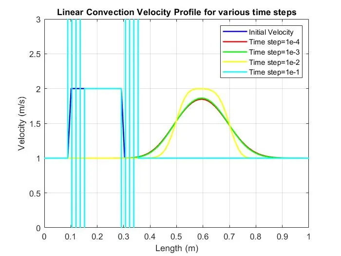
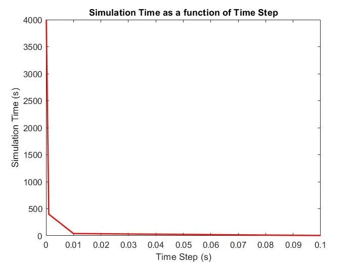
• Comparison of all test case's velocity profile at t=0.4s Variation of Simulation time as a function of time step
• 
• Figure 1 Figure 2
• The plot for a large ime step value dt=0.1, shows a blow up in solution. A comparison of the Courant number is done for this test case and an example test case dt=0.01.
• For dt=0.1:
• `c(Δt)/(Δx)=1.(0.1)/0.0127=7.87`
• Therefore, as this time step test case does not satisfy the CFL Condition, the solution is unstable.
• For dt=0.01:
• `c(Δt)/(Δx)=1.(0.01)/(0.0127)=0.787`
• Therefore, as this time step test case satisfies the CFL Condition, the solution is stable.

CONCLUSION:

• The problem statement for the solution of velocity profile at different time steps explains that, just having a smaller time step value does not affect the stability of the solution. The solution depends on the Courant number and it satisfying thr CFL condition. it is observed in Fig.1 as the time step varies, the final velocity profile is varying and very minimal difference is observed for dt=0.001 and dt=0.0001.
• It is observed in Fig.2 that, as the time step increase, the simulation time reduces. Therefore, a stable accurate scheme requiring an explicit difference solution will have very high computation time and is not feasible.