SIMULATION OF A 1D SUPER-SONIC NOZZLE FLOW USING MACORMACK METHOD

AIM:

Simulate the isentropic flow through a quasi 1D subsonic-supersonic nozzle.

Derive both the conservation and non-conservation forms of the governing equations and sovle them using the MacCormack's technique.

Determine the steady-state temperature distribution for the flow-field variables and investigate the difference between the two forms of governing equations by comparing their solutions.

Perform a grid independence test on the solution and expain all your findings.

OBJECTIVES OF THE PROJECT:

Understand and derive the conservative and non-conservative form mass conservation, momentum conservation and energy conservation equations.

Specify the initial and boundary conditions for each case.

Create a basic modular code, with function calls for each form of solution and compare the solutions using the primitive variables- mass flow rate, density, pressure, temperature and mach number.

GOVERNING EQUATIONS AND THEORY:

1D Supersonic Nozzle:

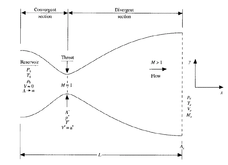
A supersonic nozzle consists of three sections, the convergent part, throat and the divergent part. In the convergent part the fluid is assumed to be entering from a reservoir and consists a Mach nnumber less than 1, therefore the flow is subsonic. At the throat, as the mass flow rate is constant, and area of cross-section decreases, velocity of the fluid increases. This leads to the Mach number reaching sonic flow at Mach number 1. In the divergent section as the area of crossection increase, but the flow variables are changed and maintained such that the flow velocity increase further more to supersonic regime where mach number is greater than 1.

Mach number can be expressed as: `M=u/c`

where `u` is the velocity of fluid and `c=sqrt(gammaRT)` is the speed of sound, `R` is the ideal gas constant and `T` is the absolute temperature.

Quasi 1D flow refers to a quasistatic flow in one-dimension, wherein the flow variables are dependent on the dimension or direction of flow. Quasistatic refers to a thermodynamic process that happens slow enough to maintain the internal equillibrium of the system.

The MacCormack method to be used is an average solution obtained from the weighted solutions of forward and backward differencing of space derivatives in the discretized equations. A time marching solution is used to obtain the solution of the problem, starting from few initial and boundary conditions which will be discussed later. In a time marching solution the current time step calculations are used to guide the way to the next time step solution.

Governing Equations:

NON-CONSERVATIVE FORM:

The following equations were extracted from Computational Fluid Dynamics Basics and Application: John D Anderson

`text(Continuity): (delrho')/(delt')=-rho'(delV')/(delx')-rho'V'(dellnA')/(delx')-V'(delrho')/(delx')`

`text(Momentum): (delV')/(delt')=-V'(delV')/(delx')-1/gamma((delT')/(delx')+(T')/(rho')(delrho')/(delx'))`

`text(Energy): (delT')/(delt')=-V'(delT')/(delx')-(gamma-1)T'((delV')/(delx')+V'(dellnA')/(delx'))`

where `rho',A',V',T',x',gamma,t'` are the nin-dimensional density, area of cross-section, velocity, temperature, length and time respectively.

The MacCormack method works with two half step calculations for the calculation of the next time step value. The 1st step called the Predictor step is a forward differencing in space for each primitive variable, wherein the above equations are used. Let us take an example of a quantity `mu` and go through the step-wise process.

`((delmu_i^(n+1/2))/(delx'))_p=(mu_(i+1)^n-mu_i^n)/(dx')`

The next step includes updating of the values:

`mu_i^(n+1/2)=mu_i^n+((delmu_i^(n+1))/(delx'))_p.dt'`

where `dt` is the ideal time step value calculated using Courant number. The time step value is derived from:

`dt=min((C.dx)/(a+V))`, where C is the Courant number, a is the speed of sound and V is the velocity of fluid. It should be noted that V and x are vectors and the calculation is done element-to-element. And then the minimum of the vector obtained is obtained as the ideal dt value.

After the Predictor method, is the Corrector Method, where the next half time step values are updated using backward differencing in space for the discretized equation.

`((delmu_i^(n+1/2))/(delx'))_c=(mu_(i)^n-mu_(i-1)^n)/(dx')`

The next step includes an average of the predictor and corrector solutions:

`((delmu_i^(n+1))/(delt'))_(avg)=1/2(((delmu_i^(n+1/2))/(delx'))_p+((delmu_i^(n+1/2))/(delx'))_c)`

The last step includes the solution update of the above computed weighted sum solution to the old values of previous time step:

`(delmu_i^(n+1))/(delt')=mu_i^n+((delmu_i^(n+1))/(delt'))_(avg).dt`

Initial and Boundary Conditions:

The initial and boundary conditions are obtained by the characterstics of the flow at the entry and exit of the domain. As the problem deals with invscid unsteady flow, the charayerstics obtained are hyperbolic in nature. A hyperbolic solution has two real characterstics drawn across the domain.

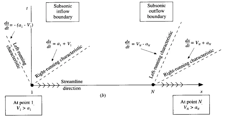
Across the domain, the characterstic lines are plotted after analyzing the direction of the fluid flow(streamline direction), the direction of the charcterstic flow and the regime of fluid flow (subsonic/supersonic). the boundary conditions obtained from method of characterstics say, at a point where one characterstic is moving into the domain, one independent flow field variable should be specified. If a characterstic is moving out of the domain, another independent flow field variable should be allowed to float as a time marching solution variable. The streamline depicted at point 1 also explains that the second flow field variable should also be specified. In the case of point N, as both the characterstics and the streamline are projecting out of the domain, therefore all the independent flow field variables will be allowed to float as a time marching solution of the calculation.

Initial Conditions:

Area of cross-section: `A=1+2.2(x-1.5)^2` for `0<=x<=3`

Density: `rho=1-0.3146x`

Temperature: `T=1-0.2314x`

Velocity: `V=(0.1+1.09x)T^(1/2)`

All the above conditions are input at t=0. The reason all the parameters are taken as a function of x is to maintain dimensional uniformity. Since the equations involved is an equation involving non-dimensional quantities, a uniform set of inputs are given.

Boundary Conditions:

Inflow: `V_1=2V_2-V_3`

Outflow:

`V_N=2V_(N-1)-V_(N-2)`

`rho_N=2rho_(N-1)-rho_(N-2)`

`T_N=2T_(N-1)-T_(N-2)`

The above conditions were formulated based on the method of characterstics discussed above.

CONSERVATIVE FORM:

The following equations were extracted for the conservation form of governing equations:

`text(Continuity): (del(rho'A'))/(delt')+(del(rho'A'V'))/(delx')=0`

`text(Momentum): (del(rho'A'V'))/(delt')+(del[rho'A'V'^2+(1/gamma)p'A'])/(delx')=(1/gamma)p'(delA')/(delx')`

`text(Energy): (del[rho'A'((e')/(gamma-1)+gamma/2V'^2)])/(delt')+(del[rho'A'V'((e')/(gamma-1)+gamma/2V'^2)+p'A'V'])/(delx')=0`

The solution is expressed in a generic form with solution vectors `U`, Flux vectors `F` and source terms `J` as:

`U_1=rho'A'`

`U_2=rho'A'V'`

`U_3=rho'A'((e')/(gamma-1)+gamma/2V'^2)`

`F_1=rho'A'V'`

`F_2=rho'A'V'+1/gammap'A'`

`F_3=rho'A'V'((e')/(gamma-1)+gamma/2V'^2)+p'A'V'`

`J_2=1/gammap'(delA')/(delx')`

Using the above terms, the governing equations are simplified to:

`(delU_1)/(delt')=-(delF_1)/(delx')`

`(delU_2)/(delt')=-(delF_2)/(delx')+J_2`

`(delU_3)/(delt')=-(delF_3)/(delx')`

The MacCormack Method will be applied to the above three equations and the solution will be obtained at each time step using the time derivatives, Predictor and Corrector steps. The boundary conditions are defined for the solution, flux and source vector. The relationship to extract the flux vector values for each time step derivative calculation is:

`F_1=U_2`

`F_2=U_2^2/U_1+(gamma-1)/(gamma)(U_3-gamma/2U_2^2/U_1)`

`F_3=gamma(U_2U_3)/(U_1)-gamma((gamma-1))/2(U_2^3)/(U_1^2)`

`J_2=(gamma-1)/gamma(U_3-gamma/2(U_2^2)/U_1)(dellnA')/(delx')`

Initial values are fed into the solution vectors, and the flux and source vectors are updated after each time-step iteration.

Initial Conditions:

`{:(rho',=,1.0),(T',=,1.0):}}text(for ) 0<=x'<=0.5`

`{:(rho',=,1.0,-,0.366(x'-0.5)),(T',=,1.0,-,0.167(x'-0.5)):}} text( for )0.5<=x'<=1.5`

`{:(rho',=,0.634,-,0.3879(x'-1.5)),(T',=,0.833,-,0.3507(x'-1.5)):}}text( for ) 1.5<=x'<=3.0`

Boundary Conditions:

Similar boundary conditions apply for the conservative form of equations:

Inflow:

`U_(1(i=1))=(rho'A')_(i=1)`

`U_(2(i=1))=2U_(2(i=2))-U_(2(i=3))`

`U_(3(i=1))=(rho'A'((e')/(gamma-1)+gamma/2V'^2))_((i=1))`

Outflow:

`U_(1(i=N))=2U_(1(i=N-1))-U_(1(i=N-2))`

`U_(2(i=N))=2U_(2(i=N-1))-U_(2(i=N-2))`

`U_(3(i=N))=2U_(3(i=N-1))-U_(3(i=N-2))`

BODY OF THE CONTENT:

CODE:

clear all, close all, clc
%1D supersonic nozzle flow simulation using MaCormack Method

%Input parameters
n=31;
x=linspace(0,3,n);
dx=x(2)-x(1);
gamma=1.4;
%CFL number 
C=0.5;
%Number of time steps
nt=1400;
t=1:1400;
%Throat index
th=(n-1)/2;

%Functions called to simulate the continuity,momentum and energy equations
%Non-Conservative
[m,M,v,T,p,rho,M_th,T_th,p_th,rho_th]=nonconservativenozzle(x,dx,n,C,nt,gamma);

%Conservative
[m_c,M_c,v_c,T_c,p_c,rho_c,M_th_c,T_th_c,p_th_c,rho_th_c]=conservativenozzle(x,dx,n,C,nt,gamma);

%Time-wise variation of density, pressure, temperature and Mach no. at
%throat

figure(3)
subplot(4,1,1)
hold on;
plot(t,rho_th)
plot(t,rho_th_c)
%legend('Non-Conservative','Conservative')
title('Time variation of quantities at throat in 1D supersonic nozzle flow')
xlabel('Time')
ylabel('Density')
grid on;

subplot(4,1,2)
hold on;
plot(t,T_th)
plot(t,T_th_c)
%legend('Non-Conservative','Conservative')
xlabel('Time')
ylabel('Temperature')
grid on;

subplot(4,1,3)
hold on;
plot(t,p_th)
plot(t,p_th_c)
%legend('Non-Conservative','Conservative')
xlabel('Time')
ylabel('Pressure')
grid on;

subplot(4,1,4)
hold on;
plot(t,M_th)
plot(t,M_th_c)
legend('Non-Conservative','Conservative')
xlabel('Time')
ylabel('Mach No.')
grid on;

%Qualitative aspect of all quantities 

figure(4)
subplot(4,1,1)
hold on;
plot(x,rho)
plot(x,rho_c)
%legend('Non-Conservative','Conservative')
title('Qualitative aspect of quantities in 1D supersonic nozzle flow')
xlabel('Length')
ylabel('Density')
grid on;

subplot(4,1,2)
hold on;
plot(x,T)
plot(x,T_c)
%legend('Non-Conservative','Conservative')
xlabel('Length')
ylabel('Temperature')
grid on;

subplot(4,1,3)
hold on;
plot(x,p)
plot(x,p_c)
%legend('Non-Conservative','Conservative')
xlabel('Length')
ylabel('Pressure')
grid on;

subplot(4,1,4)
hold on;
plot(x,M)
plot(x,M_c)
legend('Non-Conservative','Conservative')
xlabel('Length(m)')
ylabel('Mach No.')
grid on;

%Mass flowrate Final Solution Comparison

figure(5)
hold on;
plot(x,m)
plot(x,m_c)
line([0 3],[0.579 0.579])
title('Mass flow rate final solution comparison over the domain')
legend('Non-Conservative Form','Conservative Form','Exact Solution')
xlabel('Length')
ylabel('Mass Flow Rate')
grid on;

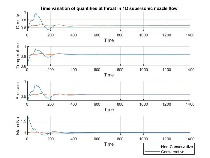
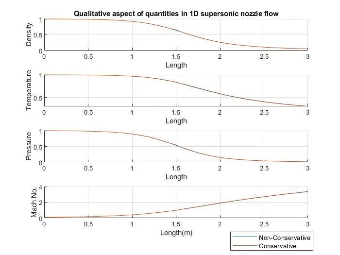
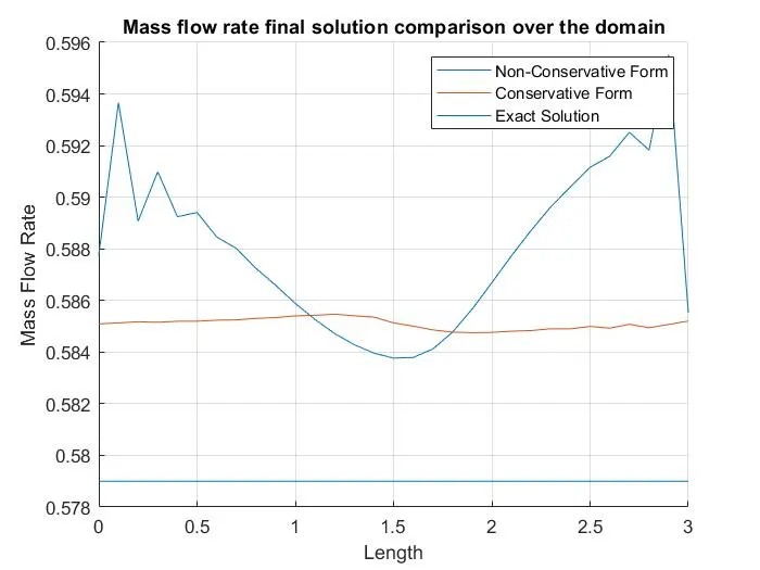
Explanation: Initially the domain variables are input and primitive variables specified. Each function is called and the respecive variables store the mach number, density, pressure, temperature and mass flow rate values across the domain. Fig.3 is plotted to show a comparison between the Conservative and Non-Conservative form of the variation of parameters as the time-steps progress. Fig.4 is plotted to show a comparison between all the primitve variables along the domain at steady state. Fig.5 is plotted to compare the final mass flow rate solution at steady state.

Function Code:

Non-Conservative Form:

%1D Supersionic Nozzle Flow Simulation- Non-Conservative
function [m,M,v,T,p,rho,M_th,T_th,p_th,rho_th]=nonconservativenozzle(x,dx,n,C,nt,gamma)

%Input paramters are specified
rho=1-0.3146*x;
T=1-0.2314*x;
v=(0.1+1.09*x).*(T.^0.5);
A=1+2.2*((x-1.5).^2);
M=v./(T.^0.5);
m=rho.*v.*A;
p=rho.*T;
%Throat index is found
th=find(A==1);

% dt calculation with Courant number at all nodes
for i=1:n
   dt_cal=(C*dx)/(sqrt(T(i))+v(i)); 
end    
%Minimum is selected as dt for solution
dt=min(dt_cal);

%Time loop for each time step calculation
for k=1:nt
    %Initial values updated
    rho_old=rho;
    v_old=v;
    T_old=T;
    m_old=m;
    p_old=p;
    M_old=M;
    
   %Predictor Method
   for j=2:n-1
      drhodx=(rho(j+1)-rho(j))/dx;
      dvdx=(v(j+1)-v(j))/dx;
      dTdx=(T(j+1)-T(j))/dx;
      dlogAdx=(log(A(j+1))-log(A(j)))/dx;
      
      drhodt_p(j)= -rho(j)*dvdx-rho(j)*v(j)*dlogAdx-v(j)*drhodx;
      dvdt_p(j)= -v(j)*dvdx-(1/gamma)*(dTdx+(T(j)/rho(j))*drhodx);
      dTdt_p(j)= -v(j)*dTdx-(gamma-1)*T(j)*(dvdx+v(j)*dlogAdx);
      
      %Solution update
      v(j)=v_old(j)+dvdt_p(j)*dt;
      rho(j)=rho_old(j)+drhodt_p(j)*dt;
      T(j)=T_old(j)+dTdt_p(j)*dt;
   end    
   
   %Corrector Method
   for j=2:n-1
      drhodx=(rho(j)-rho(j-1))/dx;
      dvdx=(v(j)-v(j-1))/dx;
      dTdx=(T(j)-T(j-1))/dx;
      dlogAdx=(log(A(j))-log(A(j-1)))/dx;
      
      drhodt_c(j)= -rho(j)*dvdx-rho(j)*v(j)*dlogAdx-v(j)*drhodx;
      dvdt_c(j)= -v(j)*dvdx-(1/gamma)*(dTdx+(T(j)/rho(j))*drhodx);
      dTdt_c(j)= -v(j)*dTdx-(gamma-1)*T(j)*(dvdx+v(j)*dlogAdx);
      
   end
   
   %Average solution update
   dvdt_avg=0.5*(dvdt_p+dvdt_c);
   drhodt_avg=0.5*(drhodt_p+drhodt_c);
   dTdt_avg=0.5*(dTdt_p+dTdt_c);
   
   %Final Solution update
   for j=2:n-1
      v(j)=v_old(j)+dvdt_avg(j)*dt;
      rho(j)=rho_old(j)+drhodt_avg(j)*dt;
      T(j)=T_old(j)+dTdt_avg(j)*dt;
   end    
   
   %Boundary Conditions
   v(1)=2*v(2)-v(3);
   v(n)=2*v(n-1)-v(n-2);
   rho(1)=1;
   rho(n)=2*rho(n-1)-rho(n-2);
   T(1)=1;
   T(n)=2*T(n-1)-T(n-2);

  %Variables updated 
  M=v./(T.^0.5);
  p=rho.*T;
  m=rho.*v.*A;

  %Throat values extracted
  T_th(k)=T(th);
  M_th(k)=M(th);
  p_th(k)=p(th);
  rho_th(k)=rho(th);
 
  %Mass flow rate at required time steps
  figure(1)
  hold on;
  if k==50
    plot(x,m,'b');
  else if k==100
    plot(x,m,'r');
  else if k==200
    plot(x,m,'g');
  else if k==400
    plot(x,m,'y');
  else if k==700
    plot(x,m,'m');
  end
  end
  end
  end
  end
end  
  title('Mass flow rate comparison at different time steps(Non-Conservative Form)') 
  xlabel('Non-dimensional Length')
  ylabel('Non-dimensional Mass Flow rate')
  legend('50 deltat','100 deltat','200 deltat','400 deltat','700 deltat')
  grid on
  axis([0 3 0 2.5]);

end    

Conservative Form:

%1D Supersionic Nozzle Flow Simulation- Conservative
function [m,M,v,T,p,rho,M_th,T_th,p_th,rho_th]=conservativenozzle(x,dx,n,C,nt,gamma)

%Initial Conditions
for i=1:length(x)
   if x(i)>=0 && x(i)<=0.5
      rho(i)=1.0;
      T(i)=1.0;
   else if x(i)>=0.5 && x(i)<=1.5
      rho(i)=1-(0.366*(x(i)-0.5));
      T(i)=1-(0.167*(x(i)-0.5));
   else if x(i)>=1.5 && x(i)<=3.0
      rho(i)=0.634-(0.3879*(x(i)-1.5));
      T(i)=0.833-(0.3507*(x(i)-1.5));
       end
       end
   end
end    
%Input values
A=1+(2.2*((x-1.5).^2));
v=0.59./(rho.*A);
p=rho.*T;
m=rho.*A.*v;
M=v./(T.^0.5);
gamma=1.4;
%Throat index
th=find(A==1);
for i=1:n
   dt_cal(i)=(C*dx)/((T(i)^0.5)+v(i)); 
end 
% dt calculation using Courant number
dt=min(dt_cal);

%Solution Vector is defragmented using the following variables
U1=rho.*A;
U2=U1.*v;
U3=rho.*A.*(T./(gamma-1)+((gamma/2).*v.^2));

%Time loop for each time step calculation
for k=1:nt
    
    %Flux Vectors
    F1=U2;
    F2=(((U2.^2)./U1)+((gamma-1)/gamma)*(U3-(gamma/2)*((U2.^2)./U1)));
    F3=((gamma.*U2.*U3)./U1)-((gamma/2)*(gamma-1).*((U2.^3)./(U1.^2)));
    
    %Intitial values noted
    U1_old=U1;
    U2_old=U2;
    U3_old=U3;
    
   %Predictor Method
   for j=2:n-1
       
      J2(j)=(1/gamma).*rho(j).*T(j).*((A(j+1)-A(j))/dx); 
       
      dU1dt_p(j)=-(F1(j+1)-F1(j))/dx;
      dU2dt_p(j)=-((F2(j+1)-F2(j))/dx)+J2(j);
      dU3dt_p(j)=-(F3(j+1)-F3(j))/dx;
      
      %Solution update
      U1(j)=U1_old(j)+dU1dt_p(j)*dt;
      U2(j)=U2_old(j)+dU2dt_p(j)*dt;
      U3(j)=U3_old(j)+dU3dt_p(j)*dt;
   end    
      %Variables are updated
      rho=U1./A;
      v=U2./U1;
      T=(gamma-1).*((U3./U1)-((gamma/2)*((U2./U1).^2)));
      p=rho.*T;
    
    %Flux updated  
    F1=U2;
    F2=(((U2.^2)./U1)+((gamma-1)/gamma)*(U3-((gamma/2)*((U2.^2)./U1))));
    F3=((gamma.*U2.*U3)./U1)-((gamma/2)*(gamma-1)).*((U2.^3)./(U1.^2));
    
   %Corrector Method
   for j=2:n-1
      J2(j)=(1/gamma).*rho(j).*T(j).*((A(j)-A(j-1))/dx); 
       
      dU1dt_c(j)=-(F1(j)-F1(j-1))/dx;
      dU2dt_c(j)=-((F2(j)-F2(j-1))/dx)+J2(j);
      dU3dt_c(j)=-(F3(j)-F3(j-1))/dx;
      
   end
   %Solution update
      dU1dt_avg=0.5*(dU1dt_p+dU1dt_c);
      dU2dt_avg=0.5*(dU2dt_p+dU2dt_c);
      dU3dt_avg=0.5*(dU3dt_p+dU3dt_c);
   
   %Final Solution update
   for j=2:n-1
      U1(j)=U1_old(j)+dU1dt_avg(j)*dt;
      U2(j)=U2_old(j)+dU2dt_avg(j)*dt;
      U3(j)=U3_old(j)+dU3dt_avg(j)*dt;
   end    
   %Variables updated
   rho=U1./A;
   v=U2./U1;
   T=(gamma-1).*((U3./U1)-((gamma/2).*((U2./U1).^2)));
   p=rho.*T;
   m=rho.*A.*v;
   M=v./(T.^0.5);
   
   %Boundary Conditions
   %Inlet
   U1(1)=rho(1)*A(1);
   U2(1)=2*U2(2)-U2(3);
   U3(1)=U1(1)*((T(1)/(gamma-1))+((gamma/2)*v(1)^2));
   
   %Outlet
   U1(n)=2*U1(n-1)-U1(n-2);
   U2(n)=2*U2(n-1)-U2(n-2);
   U3(n)=2*U3(n-1)-U3(n-2);
   
   %Throat values
   v_th(k)=v(th);
   M_th(k)=M(th);
   T_th(k)=T(th);
   p_th(k)=p(th);
   rho_th(k)=rho(th);
   
   %Mass flow rate at required time steps
   figure(2)
   hold on;
   if k==50
       plot(x,m,'b')
   else if k==100
       plot(x,m,'r')
   else if k==200
       plot(x,m,'g')
   else if k==400
       plot(x,m,'y')    
   else if k==700
       plot(x,m,'m')
       end
       end
       end
   end
   end   
end
   title('Mass flow rate comparison at different time steps(Conservative Form)')
   xlabel('Length')
   ylabel('Mass flow rate')
   legend('50 deltat','100 deltat','200 deltat','400 deltat','700 deltat')
   axis([0 3 0.4 1.6])
   grid on
end    

Function Code Explaination: The initial conditions are input based on the form of equations. The ideal time step is calculated using the Courant number formula. A time loop is run for 1400 time steps and in each loop, the predictor and corrector steps are computed over the domain of the 1D flow. the throat variable values are updated at each step, and the desired time step mass flow rates are plotted.

OUTPUT:

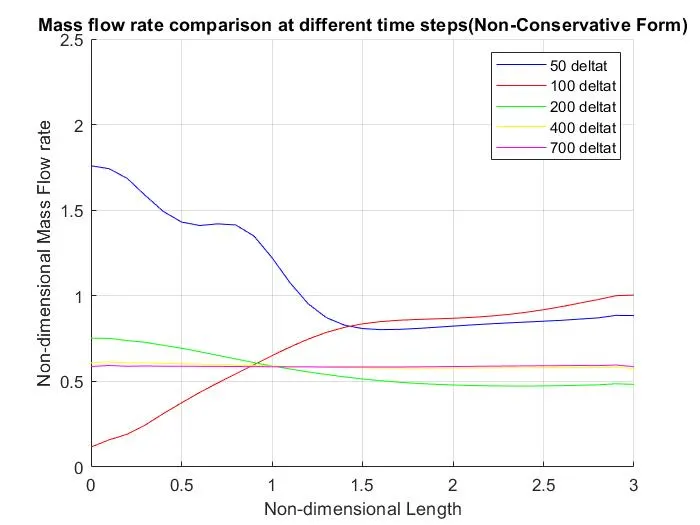
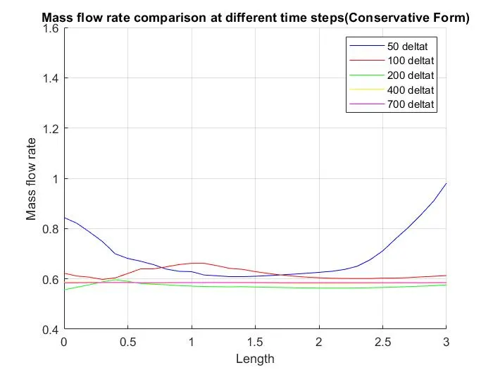
The below figures represent the conservative and non-conservative form of solution for number of grid points,n=31.

GRID DEPENDENCE TEST:

The number of nodes is changed in the above program to observe the change in solution. The " ' " symbol on each of the headings represent the non-dimensional form of the primitive variables.

Below are tabulated comparison of the non-dimensional primitive variable values at steady state at the throat of nozzle.

	Density (`rho'`)	Temperature (`T'`)	Pressure (`p'`)	Mach No. (`M`)
Exact Analytical solution	0.634	0.833	0.528	1.00
Non-conservative numerical solution (n=31)	0.639	0.836	0.534	0.999
Conservative numerical solution (n=31)	0.652	0.841	0.548	0.978
Non-conservative numerical solution (n=61)	0.637	0.835	0.532	0.999
Conservative numerical solution (n=61)	0.639	0.836	0.534	0.998

The effect of CFL number is obsereved as in, how the time step is varied and the successive solutions in the time loop (n=31). The below are the comparisons for Non-conservative form of solution, as in the previous table it is clear that its solution is closer to the analytical solution.

CFL Number	Density (`rho'`)	Temperature (`T'`)	Pressure (`p'`)	Mach No. (`M`)
Exact solution	0.634	0.833	0.528	1.00
C=0.5	0.639	0.836	0.534	0.999
C=0.7	0.639	0.836	0.535	0.999
C=0.9	0.639	0.837	0.535	0.998
C=1.1	Solution blows up/ Unstable	Solution blows up/ Unstable	Solution blows up/ Unstable	Solution blows up/ Unstable

CONCLUSION:

The mass flow rate comparison of both the forms of solutions show that, the conservative form is more stable and closer to the exact analytical solution.

The time variation of the primitive variables show that the non-conservative form portrays few disrepencies and then stablizies.

The qualitative aspect of both the forms in the domain, at steady state are almost similar.

The conservative form's mass flow rate solution reaches closer to the exact solution at 50 time step mark, than that of non-conservative form.

The grid dependence test shows that the steady state solutions for the throat values of primitive variables are closer for non-conservative solution. Increasing the number of grid points is improving the solution for both conservative and non-conservative forms.

Increasing the CFL number does not show any improvment in the non-dimensional primitive solutions at the throat for non-conservative form solution. And the solution blows up at Courant number=1.1.

Therefore the best solution cannot be decided as, non-conservative form gives better solutions for primitive variables at the throat, but computation time and consistent stability of solution is maintained by conservative form.