CFD Simulation comparing Steady and Unsteady flow over a cylinder using ANSYS Fluent

STEADY VS UNSTEADY FLOW OVER A CYLINDER

AIM:

Simulate the flow over a cylinder and explain the phenomenon of Karman vortex street.

Simulate the flow with the steady and unsteady case and calculate the Strouhal Number for Re= 100.

Calculate the coefficient of drag and lift over a cylinder by setting the Reynolds number to 10,100,1000,10000 & 100000. (Run with a steady solver). Discuss the effect of Reynolds number on the coefficient of drag. [ Results should be validated with any standard literature and error should be within 5 %]

INTRODUCTION:

One important class of fluid flow phenomena concerns the relative motion Between a fluid and the object submerged in it. The flow of air past a telephone wire or a bridge or the motion of an aircraft in a stationary atmosphere are some examples. The last flow situation is unaltered if the reference system with the aircraft is fixed, so that it appears stationary with air blowing past with the same relative velocity. An idealized geometry of a long circular cylinder is considered for understanding such flow phenomena.

GOVERNING EQUATIONS AND THEORY:

Flow visualization is used to understand the flow past a long circular cylinder held with its axis normal to a steady stream. A direct experimental method involves introduction of colored fluid at select points upstream of the cylinder and photographically records the motion of the particles.

As the flow velocity or the Reynolds number increases, changes are observed in the flow visualization mainly accounting to drag vs velocity curve. At very low values of Reynolds Number (Re<<1), the lines indicating the paths of the fluid are shown in the figure below. The pattern is symmetrical.Velocity of fluid decreases as it approaches the body and becomes zero at contact with the cylinder. This point is called STAGNATION POINT. The velocity increases from A to B and is maximum at B, and later decelerates to C (v=0), and accelerates further downstream.

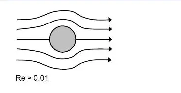
Fig. 1 Flow over cylinder at low Re

As the flow velocity and Re increase, a development of fore-and-aft symmetry is observed. Two small regions are formed just behind the cylinder in which the fluid does not flow downstream as it does elsewhere, but whirls around in closed paths. These regions of recirculating flows are called ATTACHED EDDIES. One consequence of this phenomena is that the flow no longer follows the contour of the body and is said to be SEPARATED. Another major effect that the increasing Re has on the flow picture is the modification of the region of disturbance to the flow stream. The distributed region upstream of the body and on its sides contract, while it elongates in the downstream direction. This region of disturbance downstream is termed WAKE.

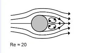
Fig. 2 Attached Eddies formation at Re=40

As Re is further increased the size of the two attached eddies increases. These eddies make the flow unstable, and consequently when the Re exceeds a value (40) the eddies are shed from the surface and swept downstream. As the eddy shed and swept away, new eddies are formed, shed and swept downstream. The eddies on either side of the cylinder shed alternatively and create an unsteady, albeit periodic, wake flow. The wake of such a flow, with a series of staggered vortices shed from either side of the cylinder and swept downstream by the flow is termed as KARMAN VORTEX STREET. It is noticed that for low values of Re, the velocity at a fixed point varies almost sinusoidally, but as Re increases the periodicity is lost.

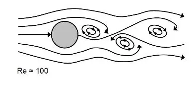
Fig. 3 Vortex Shedding at Re=100 and above

The lift coefficient is a dimensionless coefficient that relates the lift generated by a lifting body to the fluid density around the body, the fluid velocity and an associated reference area. A lifting body is a foil or a complete foil-bearing body such as a fixed-wing aircraft. `C_L` is a function of the angle of the body to the flow, its Reynolds number and its Mach number.

`C_L=L/(qS)=L/(1/2rhou^2S)=(2L)/(rhou^2S)`

where `L` is the lift force, `S` is the relevant surface area and `q` is the fluid dynamic pressure, in turn linked to the fluid density `rho`, and to the flow speed `u`.

The drag coefficient is a dimensionless quantity that is used to quantify the drag or resistance of an object in a fluid environment, such as air or water. It is used in the drag equation in which a lower drag coefficient indicates the object will have less aerodynamic or hydrodynamic drag. The drag coefficient is always associated with a particular surface area.

`C_D=(2F_d)/(rhou^2A)`

where `F_d` is the drag force, which is by definition the force component in the direction of the flow velocity, `rho` is the mass density of the fluid, `u` is the flow speed of the object relative to the fluid, `A` is the reference area.

In dimensional analysis, the Strouhal number is a dimensionless number describing oscillating flow mechanisms.

`St=(fL)/U`

where `f` is the frequency of vortex shedding, `L` is the characterstic length and `U` is the flow velocity.

For large Strouhal numbers (order of 1), viscosity dominates fluid flow, resulting in a collective oscillating movement of the fluid "plug". For low Strouhal numbers (order of 10⁻⁴ and below), the high-speed, quasi-steady-state portion of the movement dominates the oscillation. Oscillation at intermediate Strouhal numbers is characterized by the buildup and rapidly subsequent shedding of vortices. It should be noted that the Strouhal number takes into consideration the frequency count (`f=text(Number of peaks)/text(Flow time)`), which is not applicable for a steady state simultaion since no time physicality is considered in it. Strouhal number can be calculated only for transient solutions.

SOLVING AND MODELLING APPROACH:

For solving the problem statement, the following flow chart is followed:

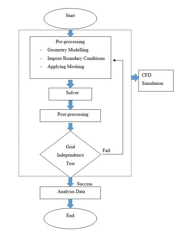
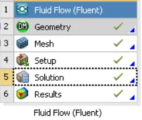
Fig. 4 ANSYS Solving Flow Chart

ANSYS involves selection of Fluent solver, input and verification of Geometry, Meshing, Setup, Solutions and Results. The Geometry is input in ANSYS Space Claim by drawing a 2D surface model of the required flow simulation. The mesh sizing and face naming is done while Meshing. The Setup section involves Mesh Checking, Turbulence Model selection, Solver type, velocity formulation and time (steady or transient state), Output report files, Material selection, Initial and Boundary conditions. The Results section is used for the visualiztion of the output in a GUI.

The modelling approach as stated in the problem statement includes both STEADY and TRANSIENT STATE simulation to observe the Strouhal Number. The solution is originally a transient state simulation output, but the desired vortex shedding can be observed in a steady state solution at higher Re values. The `k-epsilon` model is used to run the transient state simulation.

PRE-PROCESSOR AND SOLVER SETTINGS:

GEOMETRY:

The geometry is sketched in SpaceClaim. On the XZ plane, a D=2m diameter circle is drawn and enclosed with an inlet side at 10D upstream and outlet side 20D downstream. The symmetry condition used on the other two boundaries at 5D from the centre of the circle. After the geometry is drawn the circle part is deleted and the geometry is extruded outside to create a body. This is done because, now all the fluid flow is being visualized in the body left, and that is what is required for the simulation.

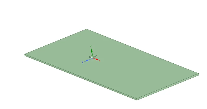
Fig. 5 Geometry of the simulation body

MESH:

The Meshing tab is opened, and when Generate Mesh is used, a mixture of quadrilaterals and triangles is input in the mesh domain. The Element size of Mesh is set to 0.3m. To create a uniform mesh, a New Method is inserted into the mesh and Tetrahedron method is selected. To improve the sizing on the edge od the circle, the Sizing option is inserted in the Mesh and the Number of Divisions is increased to 36, so that there exists one mesh element every `10^0` of the circle's circumference.

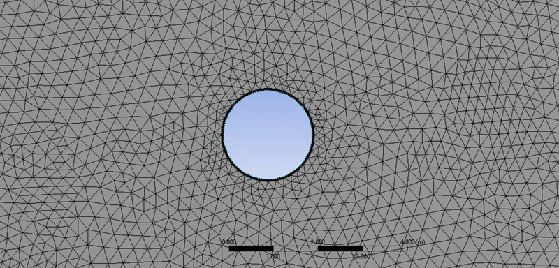
Fig. 6 Uniiform Tetrahedron Mesh

An Inflation Layer is added into the mesh to better visualize the flow at the surfacce of the circle. The First Layer thickness is set to `5e^(-3)` , the number of layer to 6 and the successive percentage increase in thickness to 20%.

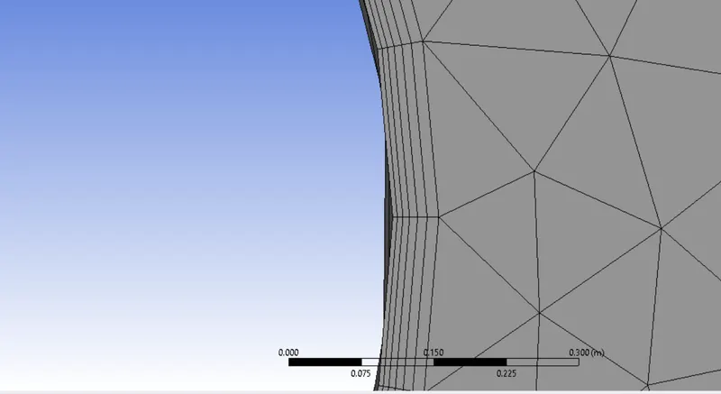
Fig. 7 Inflation Layers on the circumference of the cylinder (circle)

Later the respective sides are selected and named Inlet (upstream-left), Outlet (downstream-right), Wall (Circle circumference) and Symmetry Boundary (Above and below the circle) accordingly.

SETUP:

The simulation is run and compared for both steady and unsteady state. The Re is set to 10,100,1000,10000 and 100000 for steady state comparison and the Strouhal number is to computed for the transient state simulation (Re=100). Therefore for the respective case the solver is set to Pressure Based Type, Absolute Velocity Formulation and the Time State (Steady/Unsteady). The viscous model for both the cases is set to Laminar. A new user material is defined with `mu=0.02 Pa.s`(case specific) and `rho=1 (kg)/m^3`. The boundary conditions are set for inlet edge with velocity 1 m/s, outlet edge with pressure 1 atm. A No Slip boundary condition is employed on the cylinder wall and a Symmetry condition is set for the edges above and below the cylinder.

To observe the velocity variation a Vertex Average is plotted to a monitor point 8m (4xDiameter) downstream from the center of the cylinder. To observe the velocity development in the whole domain, a velocity contour plot is observed for each case.

It should be noted that the Convergence Criteria Check up by Fluent needs to be turned off. This is done to avoid Fluent interfere between the simulation and show a result before the desired vortices are formed.

SOLUTION:

PART I:

STEADY STATE (Re=100):

(a) (b)

(c) (d)

(e)

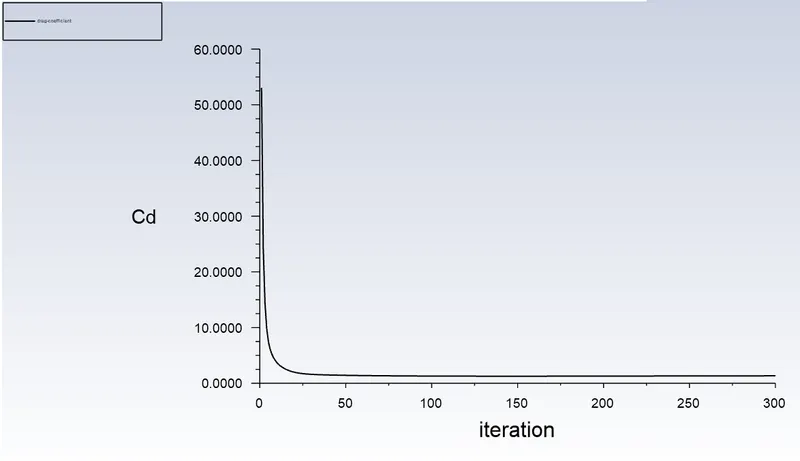
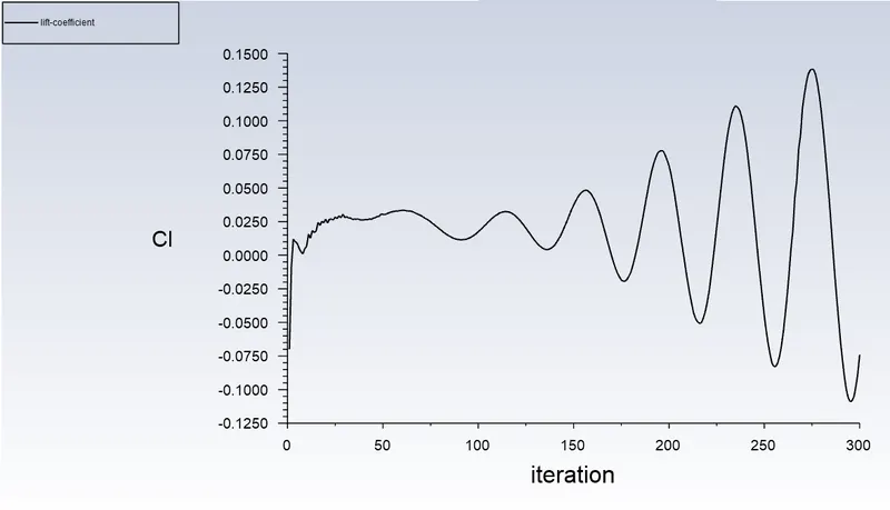
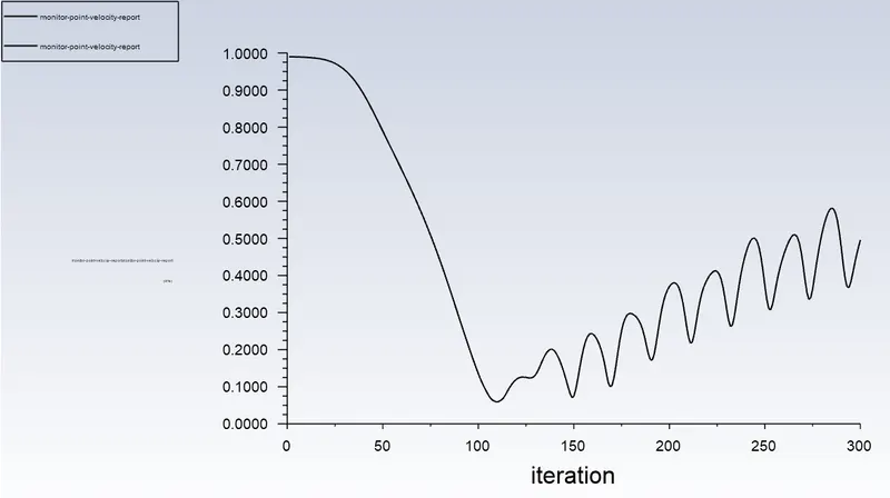
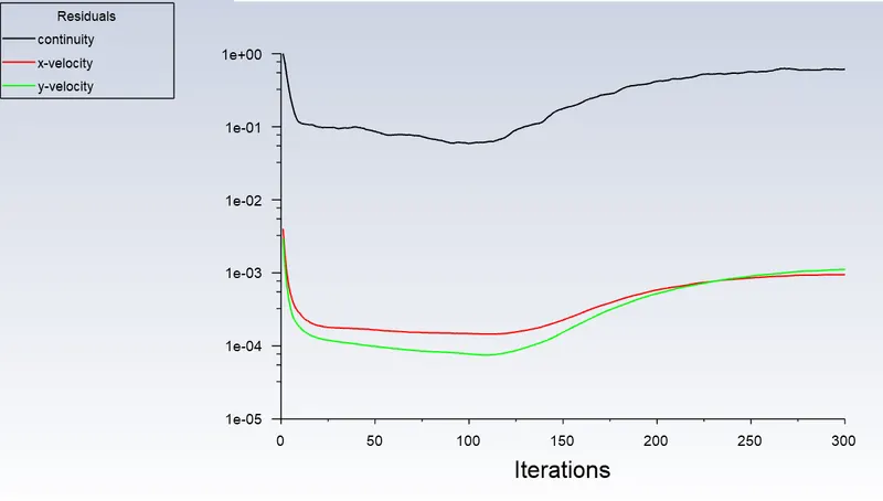
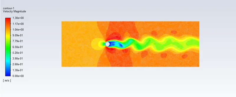
Fig. 8 (a)Drag coefficient variation as a function of number of iterations (b)Lift coefficient variation as a function of number of iterations (c) Monitor point velocity variation as a function of number of iterations (d)Residuals plot as a function of number of iterations (e) Velocity Contour at the end of simulation

The simulation was run for 300 iterations. The convergence criteria established was the plot for Residuals. Even though the continuity and velocity residual plots increased in magnitude as the vortex shedding started, they maintain a steady value and show minimal fluctuations. Therefore, they can be considered as converged for the current simulation.

TRANSIENT STATE (Re=100):

(a) (b)

(c) (d)

(e)

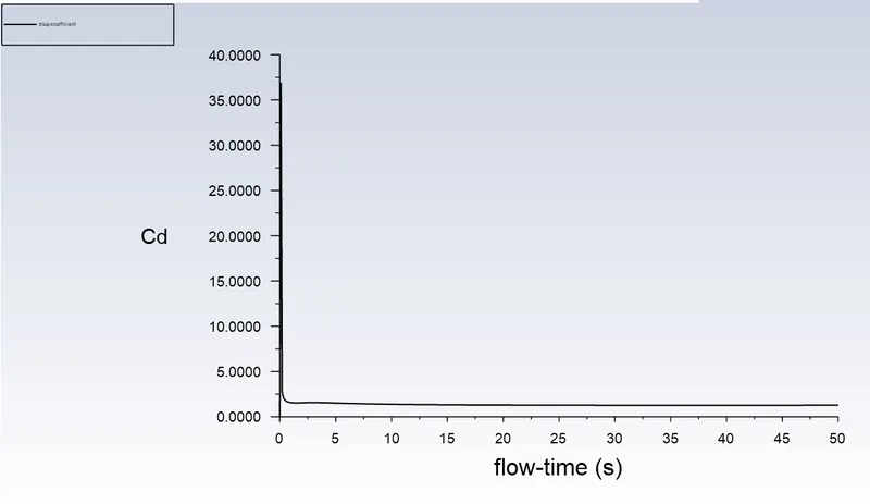
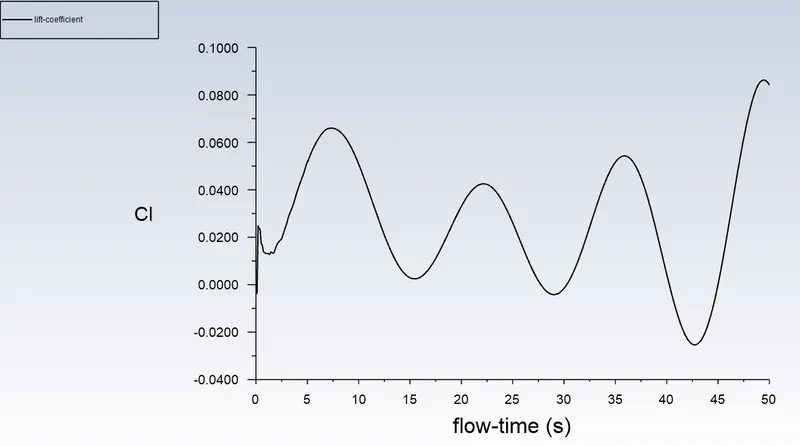
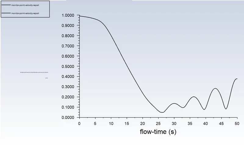
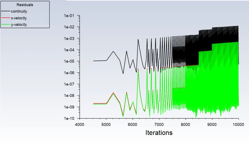
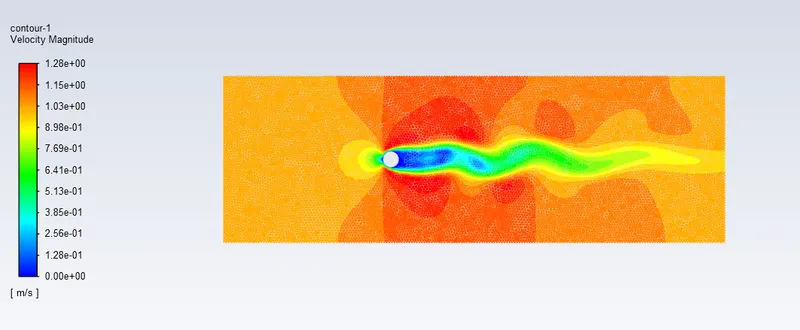
Fig. 9 (a)Drag coefficient variation as a function of number of iterations (b)Lift coefficient variation as a function of number of iterations (c) Monitor point velocity variation as a function of number of iterations (d)Residuals plot as a function of number of iterations (e) Velocity Contour at the end of simulation

The above simulation was run for a time step `dt=0.1s` and flow time of `t=50s`. Compared to the Steady state simulation, the fluctuations in the Residuals plot is even higher. The sinusidal fluctuations in the monitor point velocity are increasing gradually and are expected to stabilize after certain number of iterations.

The Strouhal Number for transient analysis:

To plot the variation of Strouhal number, Plots tab is opened, in which the FFT (Fast Fourier Transform) can be edited. The respective variable is input as "Strouhal Number" and a log plot is obtained as follows:

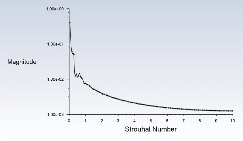
Fig. 10 Strouhal Number variation as a function of time

The values are recorded in a file format, opened in Excel to tabulate an average. The final Strouhal Number obtained is:

`St=5e^(-1)`

Comparing the simulation end state results:

	STEADY	UNSTEADY
Number of iterations/flow time	300 iterations	50s flow time
Drag coefficient `C_d`	1.337	1.283
Lift Coefficient `C_l`	-0.074	0.084
Velocity at monitor point (x=8m from centre)	0.496 m/s	0.377 m/s

PART II:

STEADY STATE (`Re=10`):

(a) (b)

(c) (d)

(e)

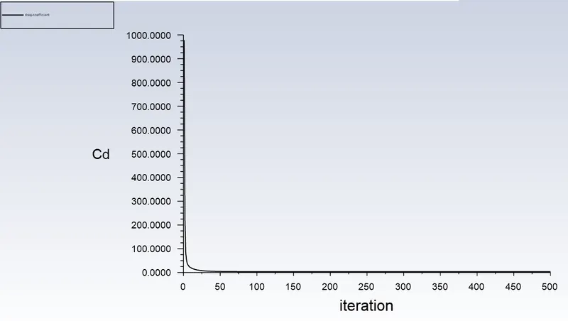
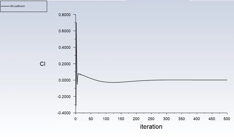
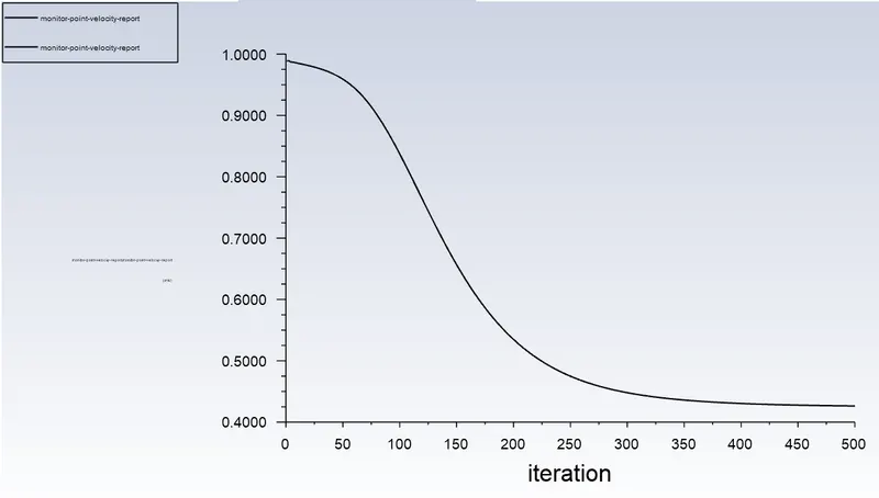
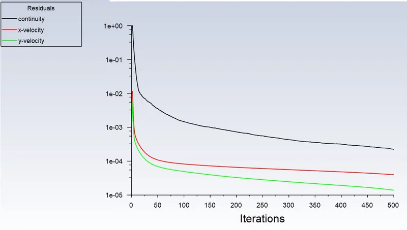
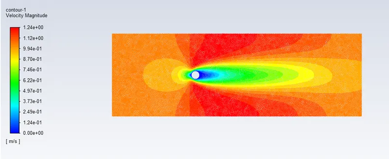
Fig. 11 (a)Drag coefficient variation as a function of number of iterations (b)Lift coefficient variation as a function of number of iterations (c) Monitor point velocity variation as a function of number of iterations (d)Residuals plot as a function of number of iterations (e) Velocity Contour at the end of simulation

The residuals are stable and reducing gradually. No vortex shedding is observed. The flow has not developed enough to show any effects on the outlet boundary. The flow can be called Attached.

STEADY STATE (`Re=100`):

(a) (b)

(c) (d)

(e)

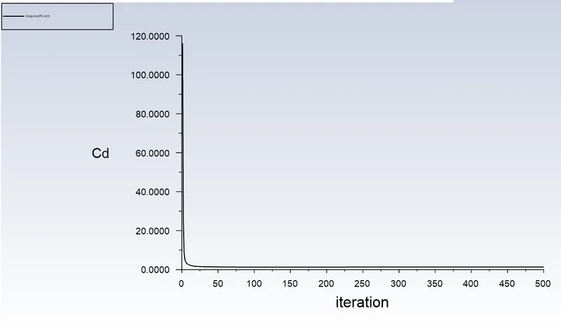
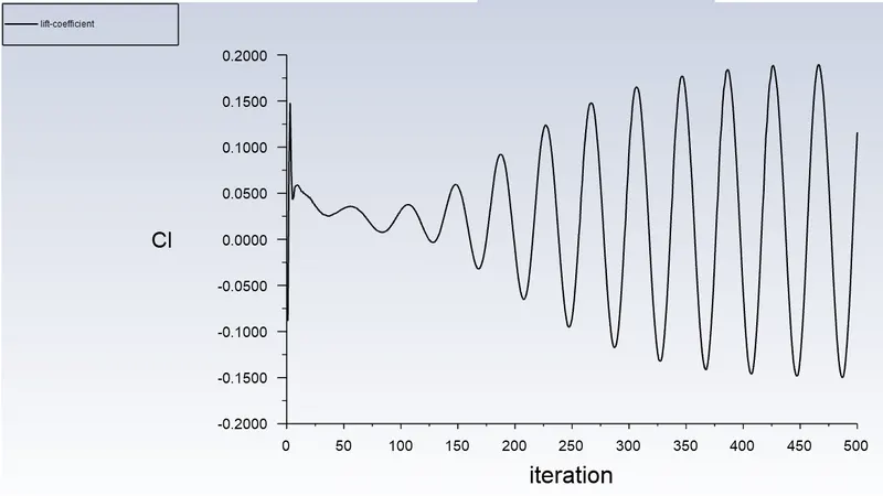
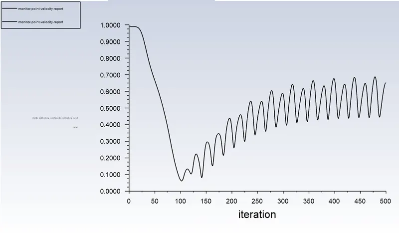
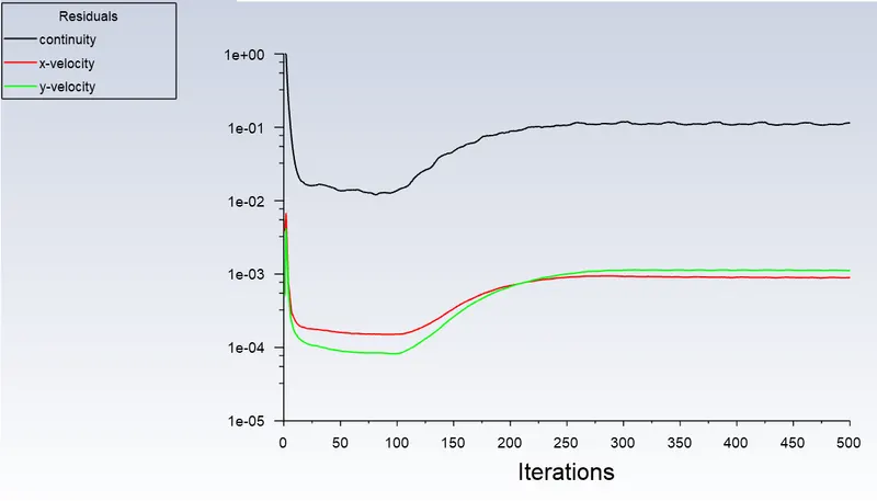
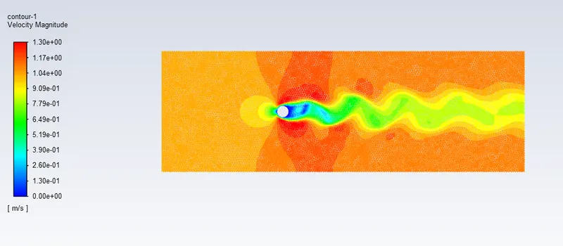
Fig. 12 (a)Drag coefficient variation as a function of number of iterations (b)Lift coefficient variation as a function of number of iterations (c) Monitor point velocity variation as a function of number of iterations (d)Residuals plot as a function of number of iterations (e) Velocity Contour at the end of simulation

Vortex shedding can be observed at this Reynolds number value. Uniform oscillation frequency is observed in the monitor point's velocity variation. The residuals have stabilized at higher values.

STEADY STATE (`Re=10^3`):

(a) (b)

(c) (d)

(e)

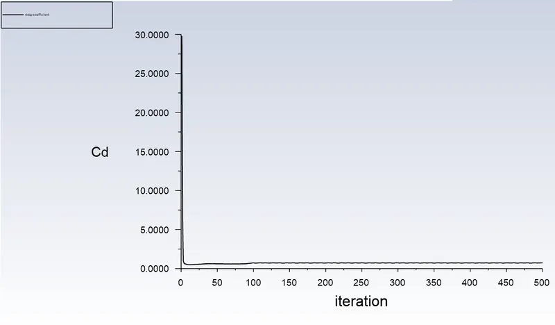
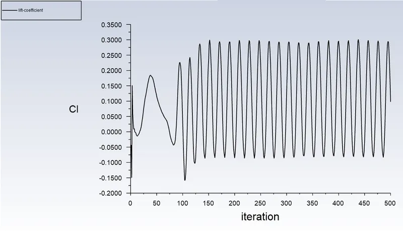
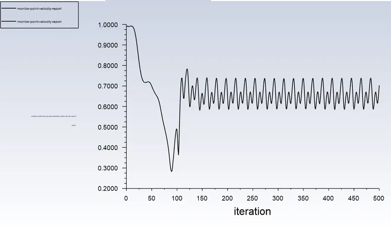
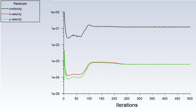
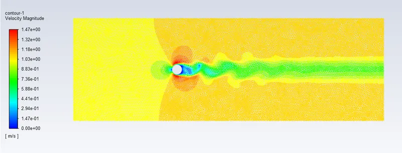
Fig. 13 (a)Drag coefficient variation as a function of number of iterations (b)Lift coefficient variation as a function of number of iterations (c) Monitor point velocity variation as a function of number of iterations (d)Residuals plot as a function of number of iterations (e) Velocity Contour at the end of simulation

It can be observed that after a certain length downstream from cylinder, the flow charcterstics dominate the viscous characterstics and the vortices vanish.

STEADY STATE (`Re=10^4`):

(a) (b)

(c) (d)

(e)

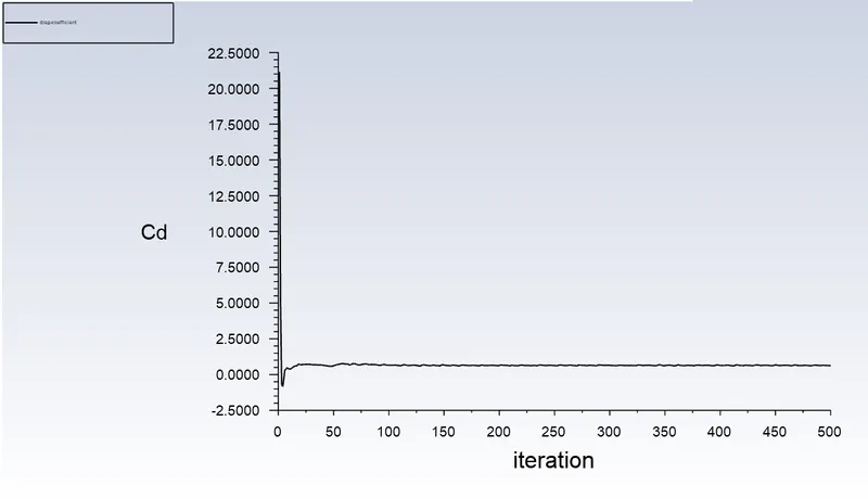
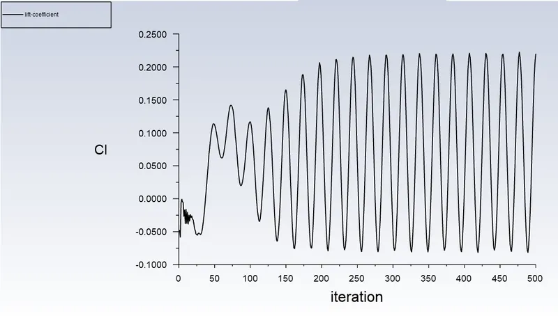
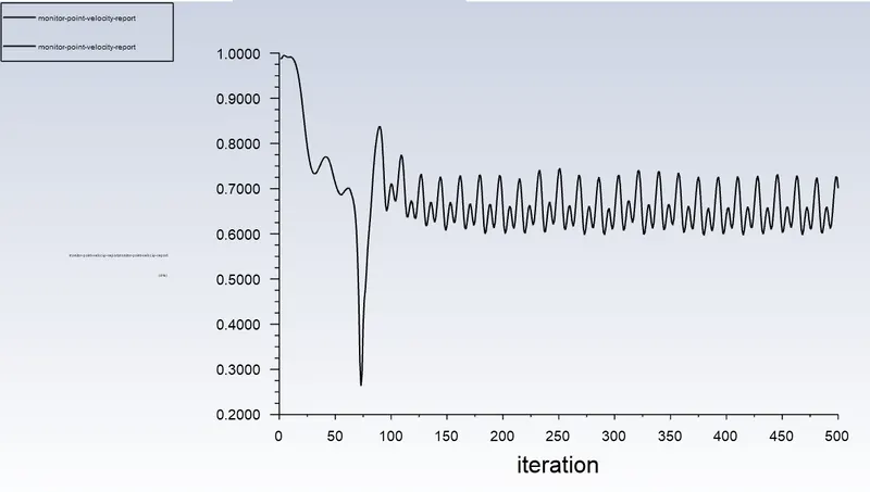
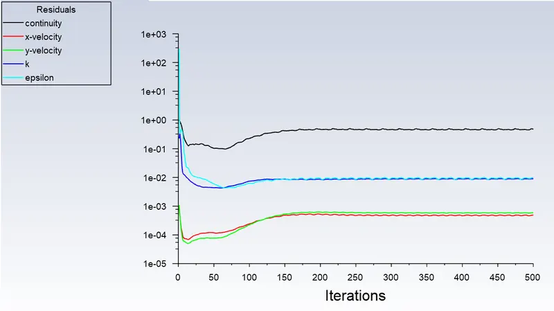
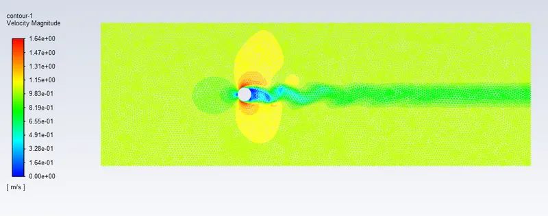
Fig. 14 (a)Drag coefficient variation as a function of number of iterations (b)Lift coefficient variation as a function of number of iterations (c) Monitor point velocity variation as a function of number of iterations (d)Residuals plot as a function of number of iterations (e) Velocity Contour at the end of simulation

It can be observed that the vortex shedding frequency is lower than the previous case, and the amplitude of the oscillating vertices has also reduced.

STEADY STATE (`Re=10^5`):

(a) (b)

(c) (d)

(e)

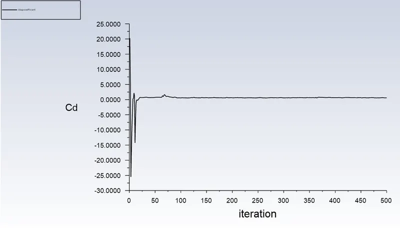
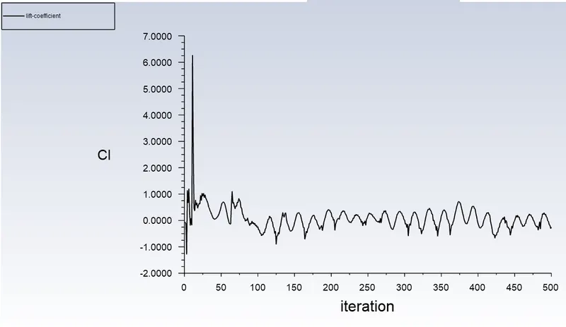
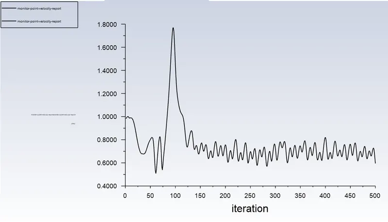
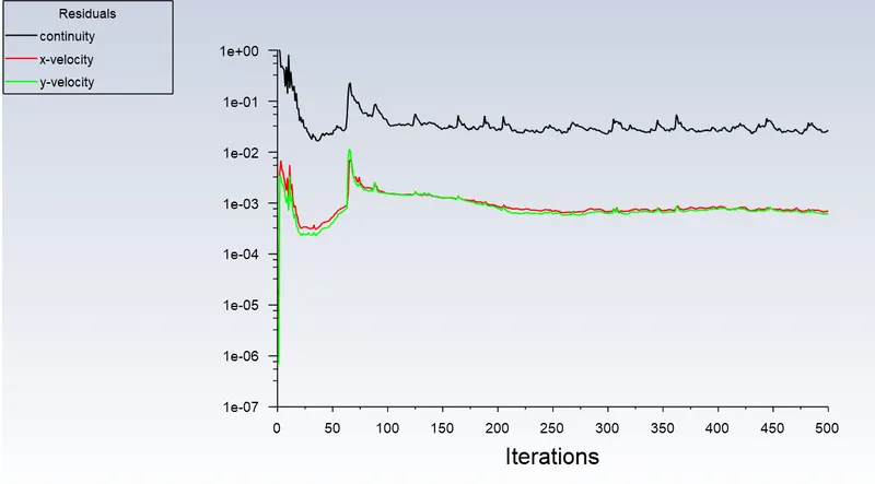
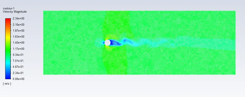
Fig. 15 (a)Drag coefficient variation as a function of number of iterations (b)Lift coefficient variation as a function of number of iterations (c) Monitor point velocity variation as a function of number of iterations (d)Residuals plot as a function of number of iterations (e) Velocity Contour at the end of simulation

In this case, the distinction between the velocities is very difficult. The flow velocity is high enough to dominate and completely dissolve the viscous effects.

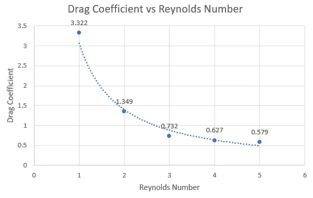
A tabulated comparison of all the steady state cases for 500 iterations is given below:

	Drag Coefficient `C_d`	Lift Coefficient `C_l`	Monitor Point Velocity (m/s)
`Re=10`	3.322	0.001	0.426
`Re=10^2`	1.349	0.116	0.650
`Re=10^3`	0.732	0.097	0.703
`Re=10^4`	0.627	0.011	0.700
`Re=10^5`	0.579	0.253	0.595

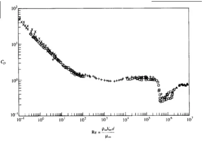
The comparison between Velocity Drag coefficient and Reynolds number is done below:

(a) (b)

Fig. 16 (a) Drag Coefficient vs log Reynolds Number (b) Variation of cylinder drag coefficient with Reynolds number (Theoretical).

It can be observed that as the Reynolds Number increases, the Drag coefficient decreases.

CONCLUSION:

For Re=100, the comparison between the steady state and transient state simulation states that: The viscous effects are diminished in the transient state analysis as the amplitude of the vortex oscillations is low.

For the steady state part 2 analysis, the Reynolds number is inversely proportional to the drag coefficient and lift coefficient.

Convergence can also be tested based on the stability of the Residual plots.

As the Reynolds number increases for the steady state analysis, the vortex shedding is reduced due to the dominance of flow characterstics over viscous effects.

RESOURCES:
Source: Experimental data from Incompressible Flow, Wiley-Interscience, New York (1984).