Taylor Table Method for solving Numerical solution

TAYLOR TABLE METHOD

AIM:

• Derive a 4^th Order approximation of the second order derivative for a central differencing scheme, Skewed left-sided difference and Skewed right-sided difference.
• Also prove that your skewed schemes are 4^th Order accurate.
• Compare the absolute error plots for the above schemes for the function =exp(x)*cos(x).
• Describe why a skewed scheme is useful, and what can a skewed scheme do which a central difference scheme cannot do.

OBJECTIVES OF THE PROJECT:

• Apply Taylor Table method to compute coefficients for all the approximation schemes.
• Derive the coefficients of higher order terms to prove the order of accuracy of skewed schemes.
• Formulate a vector computing the absolute error between the analytical solution and numerical solution.
• Plot a loglog graph to compare the error vectors.

GOVERNING EQUATIONS:

1. 4^th Order approximation of a second order derivative using central difference scheme

In this scheme, a stencil including points (i-2),(i-1),(i),(i+1) and (i+2) is used.

Firstly, the desired derivative is written as a function of all the stencil points.

`(delta^2f)/(deltax^2)=af(x−2)+bf(x−1)+cf(x)+df(x+1)+ef(x+2)`_____(1)

The Taylor Table method is applied:

	`f(x)`	`(f'(x))/(Deltax)`	`f''(x)Deltax^2`	`f^(iii)(x)Deltax^3`	`f^(iv)(x)Deltax^4`
`af(x-2)`	`a`	`-2a`	`(2^2a)/(2!)`	`(-2^3a)/(3!)`	`(2^4a)/(4!)`
`bf(x-1)`	`b`	`-b`	`b/(2!)`	`-b/(3!)`	`d/(4!)`
`cf(x)`	`c`	`0`	`0`	`0`	`0`
`df(x+1)`	`d`	`d`	`d/(2!)`	`d/(3!)`	`d/(4!)`
`ef(x+2)`	`e`	`2e`	`(2^2e)/(2!)`	`(2^3e)/(3!)`	`(2^4e)/(4!)`
Sum=	`0`	`0`	`1`	`0`	`0`

Each of the term in the 1st column is expanded using Taylor Series and the appropriate coefficient is assigned to the function values. The sum of the respective derivatives are written in the last row. The reason the second derivative sum is 1, is because the final approximation needed is for 2nd derivative of the function. And since 5 coeffficients are used-a,b,c,d,e, 5 equations are used upto `f^(iv)(x)`. Arranging the equations in matrix form as a set of linear equations:

`[[1,1,1,1,1],[-2,-1,0,1,2],[4,1,0,1,4],[-8,-1,0,1,8],[16,1,0,1,16]][(a),(b),(c),(d),(e)]=[(0),(0),(2/(Deltax^2)),(0),(0)]`

Considering the above matrix as `AX=B`, the solution for the matrix is `X=A^-1B`. This can be solved using `text(linsolve(A,B))` command in MATLAB. Therefore, the final coefficients obtained are:

`a=-0.0833/(Deltax^2),b=1.333/(Deltax^2),c=-2.5000/(Deltax^2),d=1.3333/(Deltax^2),e=-0.08333/(Deltax^2)`

The above coefficients will be applied in Eqn.1 for the numerical approximation.

2. 4^th Order approximation of a second order derivative using skewed left-sided difference scheme

In this scheme, a stencil including points (i-5),(i-4),(i-3),(i-2),(i-1) and (i) is used.

Firstly, the desired derivative is written as a function of all the stencil points.

`(delta^2f)/(deltax^2)=af(x)+bf(x-1)+cf(x-2)+df(x-3)+ef(x-4)+gf(x-5)`_____(2)

The Taylor Table Method is applied:

	`f(x)`	`f'(x)Deltax`	`f''(x)Deltax^2`	`f^(iii)(x)Deltax^3`	`f^(iv)(x)Deltax^4`	`f^(v)(x)Deltax^5`	`f^(vi)(x)Deltax^6`
`af(x)`	`a`	`0`	`0`	`0`	`0`	`0`	`0`
`bf(x-1)`	`b`	`-b`	`(b)/(2!)`	`(-b)/(3!)`	`(b)/(4!)`	`(-b)/(5!)`	`b/(6!)`
`cf(x-2)`	`c`	`-2c`	`(2^2c)/(2!)`	`(-2^3c)/(3!)`	`(2^4c)/(4!)`	`(-2^5c)/(5!)`	`(2^6c)/(6!)`
`df(x-3)`	`d`	`-3d`	`(3^2d)/(2!)`	`(-3^3d)/(3!)`	`(3^4d)/(4!)`	`(-3^5d)/(5!)`	`(3^6d)/(6!)`
`ef(x-4)`	`e`	`-4e`	`(4^2e)/(2!)`	`(-4^3e)/(3!)`	`(4^4e)/(4!)`	`(-4^5e)/(5!)`	`(4^6e)/(6!)`
`gf(x-5)`	`g`	`-5g`	`(5^2g)/(2!)`	`(-5^3g)/(3!)`	`(5^4g)/(4!)`	`(-5^5g)/(5!)`	`(5^6g)/(6!)`
Sum=	`0`	`0`	`1`	`0`	`0`	`0`	To be found

Each of the term in the 1st column is expanded using Taylor Series and the appropriate coefficient is assigned to the function values. The sum of the respective derivatives are written in the last row. The reason the second derivative sum is 1, is because the final approximation needed is for 2nd derivative of the function. And since 6 coefficients are used- a,b,c,d,e,g, 6 equation are used upto `f^(vi)(x)`. Arranging the equations in matrix form as a set of linear equations:

`[[1,1,1,1,1,1],[0,-1,-2,-3,-4,-5],[0,1,2^2,3^2,4^2,5^2],[0,-1,-2^3,-3^3,-4^3,-5^3],[0,1,2^4,3^4,4^4,5^4],[0,-1,-2^5,-3^5,-4^5,-5^5]][(a),(b),(c),(d),(e),(g)]=[(0),(0),(2/(Deltax^2)),(0),(0),(0)]`

Solving the above set of equations:

`a=3.75000/(Deltax^2),b=-12.8333/(Deltax^2),c=17.8333/(Deltax^2),d=-13.0000/(Deltax^2),e=5.08333/(Deltax^2),g=-0.83333/(Deltax^2)`

The above coefficients will be applied in Eqn.2 for the numerical approximation.

The to be found section left at the coefficient sum of `f^(vi)(x)` is to find the order of the approximation. When the computed coefficients are input into this sum, i.e.

sum of coefficients of `f^(vi)(x)=b/(6!)+(2^6c)/(6!)+(3^6d)/(6!)+(4^6e)/(6!)+(5^6g)/(6!)`

when the coefficients are input, the sum= `-0.76f^(vi)(x)Deltax^4`. Therefore the sum of the above taylor table becomes:

`(delta^2f)/(deltax^2)=af(x)+bf(x-1)+cf(x-2)+df(x-3)+ef(x-4)+gf(x-5)=f′′(x)+O(Δx^4)`. Therefore the order of the approximation is 4.

3. 4^th Order approximation of a second order derivative using skewed right-sided difference scheme

In this scheme, a stencil including points (i+5),(i+4),(i+3),(i+2),(i+1) and (i) is used.

Firstly, the desired derivative is written as a function of all the stencil points.

`(delta^2f)/(deltax^2)=af(x)+bf(x+1)+cf(x+2)+df(x+3)+ef(x+4)+gf(x+5)`_____(3)

The Taylor Table Method is applied:

	`f(x)`	`f'(x)Deltax`	`f''(x)Deltax^2`	`f^(iii)(x)Deltax^3`	`f^(iv)(x)Deltax^4`	`f^(v)(x)Deltax^5`	`f^(vi)(x)Deltax^6`
`af(x)`	`a`	`0`	`0`	`0`	`0`	`0`	`0`
`bf(x+1)`	`b`	`b`	`(b)/(2!)`	`(b)/(3!)`	`(b)/(4!)`	`(b)/(5!)`	`b/(6!)`
`cf(x+2)`	`c`	`2c`	`(2^2c)/(2!)`	`(2^3c)/(3!)`	`(2^4c)/(4!)`	`(2^5c)/(5!)`	`(2^6c)/(6!)`
`df(x+3)`	`d`	`3d`	`(3^2d)/(2!)`	`(3^3d)/(3!)`	`(3^4d)/(4!)`	`(3^5d)/(5!)`	`(3^6d)/(6!)`
`ef(x+4)`	`e`	`4e`	`(4^2e)/(2!)`	`(4^3e)/(3!)`	`(4^4e)/(4!)`	`(4^5e)/(5!)`	`(4^6e)/(6!)`
`gf(x+5)`	`g`	`5g`	`(5^2g)/(2!)`	`(5^3g)/(3!)`	`(5^4g)/(4!)`	`(5^5g)/(5!)`	`(5^6g)/(6!)`
Sum=	`0`	`0`	`1`	`0`	`0`	`0`	To be found

Each of the term in the 1st column is expanded using Taylor Series and the appropriate coefficient is assigned to the function values. The sum of the respective derivatives are written in the last row. The reason the second derivative sum is 1, is because the final approximation needed is for 2nd derivative of the function. And since 6 coefficients are used- a,b,c,d,e,g, 6 equation are used upto `f^(vi)(x)`. Arranging the equations in matrix form as a set of linear equations:

`[[1,1,1,1,1,1],[0,1,2,3,4,5],[0,1,2^2,3^2,4^2,5^2],[0,1,2^3,3^3,4^3,5^3],[0,1,2^4,3^4,4^4,5^4],[0,1,2^5,3^5,4^5,5^5]][(a),(b),(c),(d),(e),(g)]=[(0),(0),(2/(Deltax^2)),(0),(0),(0)]`

Solving the above set of equations:

`a=3.75000/(Deltax^2),b=-12.8333/(Deltax^2),c=17.8333/(Deltax^2),d=-13.0000/(Deltax^2),e=5.08333/(Deltax^2),g=-0.83333/(Deltax^2)`

The above coefficients will be applied in Eqn.3 for the numerical approximation.

The to be found section left at the coefficient sum of `f^(vi)(x)` is to find the order of the approximation. When the computed coefficients are input into this sum, i.e.

sum of coefficients of `f^(vi)(x)=b/(6!)+(2^6c)/(6!)+(3^6d)/(6!)+(4^6e)/(6!)+(5^6g)/(6!)`

when the coefficients are input, the sum= `-0.76f^(vi)(x)Deltax^4`. Therefore the sum of the above taylor table becomes:

`(delta^2f)/(deltax^2)=af(x)+bf(x+1)+cf(x+2)+df(x+3)+ef(x+4)+gf(x+5)=f′′(x)+O(Δx^4)`. Therefore the order of the approximation is 4.

4. 2nd Order approximation of a second order derivative using central difference scheme

In this scheme, three points are included (i-1),(i+1) and (i).

To prove this we add the following Taylor Expansions:

`f(x+a)=f(x)+f′(x)Δx+f′′(x)(Deltax^2)/(2!)+....`

`f(x-a)=f(x)-f′(x)Δx+f′′(x)(Deltax^2)/(2!)-....`

Adding the two equations,

`f(x+a)+f(x-a)=2f(x)+f′′(x)Deltax^2+2f^(iv)(Deltax^4)/(4!)+....`

Sending `f(x)` term to the other side, and dividing both sides with `Deltax^2`:

`(f(x+a)-2f(x)+f(x-a))/(Deltax^2)=f′′(x)+O(Deltax^2)`_____(4)

The above computed equation gives a second order approximation of the second order derivative using a 3 point stencil.

BODY OF THE CONTENT:

MAIN CODE:

clear all,close all,clc
%Taylor Table Method 
%Analytical function=exp(x)*cos(x)
%Derivation and Error calculation of 4th Order approximation for 2nd order derivative 
x=pi/3;
dx=linspace(0,pi/4,500);
%central_diff calls a function for the computation of the central
%difference function. And stores the absolute difference between the
%numerical and analytical solution
central_diff=centraldifference(x,dx);
%skewed_right calls a function for the computation of the skewed
%right-sided difference function. And stores the absolute difference between 
%the numerical and analytical solution
skewed_right=skewedrightsided(x,dx);
%skewed_left calls a function for the computation of the skewed
%left-sided difference function. And stores the absolute difference between 
%the numerical and analytical solution
skewed_left=skewedleftsided(x,dx);

%2nd Order Central Difference approximation for 2nd Order derivative
%central2_diff calls a function for the computation of the central
%difference function(2nd Order). And stores the absolute difference between 
%the numerical and analytical solution.
central2_diff=central2diff(x,dx);

%Plotting error vs dx values
%loglog function plots a logx vs logy plot of the input paramters
loglog(dx,central_diff,'r','linewidth',2)
hold on
loglog(dx,skewed_right,'b','linewidth',2)
hold on
loglog(dx,skewed_left,'g','linewidth',2)
hold on
loglog(dx,central2_diff,'linewidth',2)
legend('4th Order Central Difference','4th Order Skewed Right-sided Difference','4th Order Skewed Right-sided Difference','2nd Order Central Difference')
xlabel('log(dx)')
ylabel('log(Absolute Error)')
title('Taylor Table Method for Numerical Approximation')     

Explaination: The code above starts with clear all, close all and clc to clear the command window, workspace and any open plots or figures. Value of 'x' is specified, the point at which the second order derivative is to be calculated. A 'dx' vector parameter is input using linspace">linspacelinspace command. This helps in gauging the error as dx values reduces. Each of the 4th Order numerical approximation functions are called and the error is stored in the stated output values- central_diff,skewed_left and skewed_right. central2_diff is a function used to call for the computation of the 2nd Order approximation for the desired derivative. In the similar fashion as the previous functions the absolute difference between the analytical and numerical solution is stored in the vector. 'loglog' command is used to plot the log(Absolute Error) vs log(dx) for each numerical solution.

CENTRAL DIFFERENCE FUNCTION (4th Order):

%Function to compute 4th order approximation using central differencing
function [output]=centraldifference(x,dx)
   %Analytical Derivative
   analytical_deri=-2*exp(x)*sin(x);
   %Derivation of Numerical solution
   %Solving the set of linear equations,following coefficients are obtained
   %XY=B. Therefore Y=inv(X).B
   X=[1,1,1,1,1;-2,-1,0,1,2;4,1,0,1,4;-8,-1,0,1,8;16,1,0,1,16];
   B=[0;0;2;0;0];
   Y=linsolve(X,B);
   %Central differencing expression obtained using Eqn.1
   for i=1:length(dx)
   central_diff(i)=(Y(1)*funcofx(x-2*dx(i))+Y(2)*funcofx(x-dx(i))+Y(3)*funcofx(x)+Y(4)*funcofx(x+dx(i))+Y(5)*funcofx(x+2*dx(i)))/(dx(i)^2);
   end
   %output stores the absolute error value between the numerical and
   %analytical solution
   output=abs(analytical_deri-central_diff);
end

The above stated function gives output of the absolute error to central_diff in the main code. The analytical derivative for the function is computed. The set of linear equations derived in theory are input and solved using command 'linsolve'. The variables a,b,c,d, and e are obtained in a column vector Y, and are input in Eqn.1 to calculate the approximation. The 'abs' command is used to calculate the absolute error between the numerical and analytical solution.

SKEWED LEFT-SIDED DIFFERENCE (4th Order):

%Function to compute 4th order approximation using skewed left-sided differencing
function [output]=skewedleftsided(x,dx)
   %Analytical Derivative
   analytical_deri=-2*exp(x)*sin(x);
   %Derivation of Numerical solution
   %Solving the set of linear equations,following coefficients are obtained 
   X=[1,1,1,1,1,1;0,-1,-2,-3,-4,-5;0,1,4,9,16,25;0,-1,-8,-27,-64,-5^3;0,1,16,81,256,5^4;0,-1,-2^5,-3^5,-4^5,-5^5];
   B=[0;0;2;0;0;0];
   Y=linsolve(X,B);
   %Skewed Left sided differencing expression obtained using Eqn.2
   for i=1:length(dx)
   skewedleft_diff(i)=(Y(1)*funcofx(x)+Y(2)*funcofx(x-dx(i))+Y(3)*funcofx(x-2*dx(i))+Y(4)*funcofx(x-3*dx(i))+Y(5)*funcofx(x-4*dx(i))+Y(6)*funcofx(x-5*dx(i)))/(dx(i)^2);
   end
   %output stores the absolute error value between the numerical and
   %analytical solution
   output=abs(analytical_deri-skewedleft_diff);
end

The above stated function gives output of the absolute error to skewed_left in the main code. The analytical derivative for the function is computed. The set of linear equations derived in theory are input and solved using command 'linsolve'. The variables a,b,c,d,e and g are obtained in a column vector Y, and are input in Eqn.2 to calculate the approximation. The 'abs' command is used to calculate the absolute error between the numerical and analytical solution.

SKEWED RIGHT-SIDED DIFFERENCE (4th Order):

%Function to compute 4th order approximation using skewed right-sided differencing
function [output]=skewedrightsided(x,dx)
   %Analytical Derivative
   analytical_deri=-2*exp(x)*sin(x);
   %Derivation of Numerical solution
   %Solving the set of linear equations,following coefficients are obtained 
   X=[1,1,1,1,1,1;0,1,2,3,4,5;0,1,4,9,16,25;0,1,8,27,64,5^3;0,1,16,81,256,5^4;0,1,2^5,3^5,4^5,5^5];
   B=[0;0;2;0;0;0];
   Y=linsolve(X,B);
   %Skewed Right sided differencing expression obtained using Eqn.3
   for i=1:length(dx)
   skewedright_diff(i)=(Y(1)*funcofx(x)+Y(2)*funcofx(x+dx(i))+Y(3)*funcofx(x+2*dx(i))+Y(4)*funcofx(x+3*dx(i))+Y(5)*funcofx(x+4*dx(i))+Y(6)*funcofx(x+5*dx(i)))/(dx(i)^2);
   end
   %output stores the absolute error value between the numerical and
   %analytical solution
   output=abs(analytical_deri-skewedright_diff);
end

The above stated function gives output of the absolute error to skewed_right in the main code. The analytical derivative for the function is computed. The set of linear equations derived in theory are input and solved using command 'linsolve'. The variables a,b,c,d,e and g are obtained in a column vector Y, and are input in Eqn.3 to calculate the approximation. The 'abs' command is used to calculate the absolute error between the numerical and analytical solution.

CENTRAL DIFFERENCE FUNCTION (2nd Order):

%Function to compute 2nd order approximation using Central differencing
function [output]=central2diff(x,dx)
   %Analytical Derivative
   analytical_deri=-2*exp(x)*sin(x);
   %Derivation of Numerical solution
   %Skewed Right sided differencing expression obtained using Eqn.4
   for i=1:length(dx)
   central2_diff(i)=(-2*funcofx(x)+funcofx(x+dx(i))+funcofx(x-dx(i)))/(dx(i)^2);
   end
   %output stores the absolute error value between the numerical and
   %analytical solution
   output=abs(analytical_deri-central2_diff);
end

The above stated function gives output of the absolute error to central2_diff in the main code. The analytical derivative for the function is computed. Eqn.3 is used to compute the numerical approximation. The 'abs' command is used to calculate the absolute error between the numerical and analytical solution.

OUTPUT:

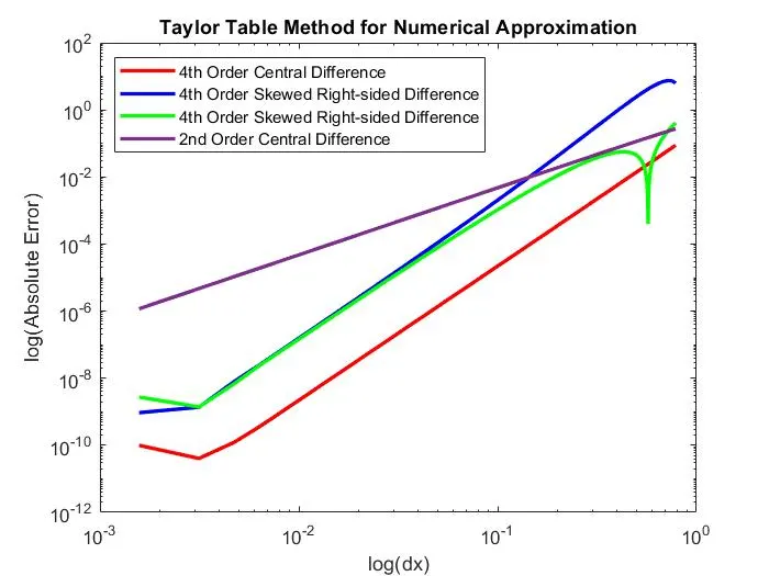
Figure 1

The above figure shows a log vs log plot between the absolute error and cell size dx.

ANSWERS TO QUESTIONS:

Q:Describe why a skewed scheme is useful? What can a skewed scheme do that a CD scheme cannot?

A: In a case where higher order derivatives are to be computed at boundary/corner points, i.e. when data of flow exists only on one side of the domain, skewed scheme can be used. This happens because central difference scheme requires data from both sides of the corner, which cannot be obtained. This scheme might not give as accurate results as central difference scheme, but an acceptable range of results are produced.

CONCLUSION:

• It can clearly be observed in Figure 1 that all the 4th order approximation functions compute lower error as cell size reduces when compared to the 2nd order central differencing approximations.
• Among the 4th order approximations central differencing computation shows significantly better results than the skewed computations. This is happeing because the central difference scheme accepts data from points on both left and right side,i.e. the previous node data and next node data points are considered in the computation of the derivative. If either of the skewed computation schemes are observed, the data is extracted only from one side. This is not an accurate way to compute the derivative of the function.