Numerical Discretization - Basics

DISCRETIZATION BASICS

AIM:

• Write a program that compares the first, second and fourth order approximations of the first derivative against the analytical or exact derivative.

OBJECTIVES OF THE PROJECT:

• To understand the theory and derivation of first, second and forth order numerical approximations of a function.
• Compute the numerical solutions using the derived formulae for each approximation.
• Get absolute error between the numerical and exact solution for different regions and understand the plot.

GOVERNING EQUATIONS AND THEORY:

• The function given for the problem statement is `f(x)=sinx/x^3`
• Taylor Series expansion states that:
• `f(x+a)=f(x)+f'(a)Deltax+f''(a)Deltax^2/(2!)+....`
• where `Deltax` is the difference between 'x' and 'x+a'. After getting the `f(x)` term on left hand side and dividing both sides with `Deltax`.
• `(f(x+a)−f(x))/(Deltax)=f'(a)+f''(a)Deltax/(2!)+....`
• For a very small value of `Deltax` the higher order terms can be neglected and the approximation becomes a first order approximation. This is because the largest error term is a multiple of `Deltax^1`.
• Therefore,
• `(f(x+a)-f(x))/(Deltax)=f'(a)+O(Deltax)`_____(1)
• The above equation is a forward differencing numerical approximation of the function. When similar taylor series expansion is applied to `f(x-a)` , a backward differencing numerical approximation is observed.
• `(f(x-a)-f(x))/(Deltax)=-f'(a)+O(Deltax)`_____(2)
• Both the above approximations are first order, and hence use only 2 points on the stencil for computation. If Eqn.1 and 2 are added and arranged to give ,
• `f'(a)=(f(x+a)−f(x−a))/(2Deltax)+O(Deltax^2)`
• This is a second order derivative, which can be proven by expanding both the `f(x+a)` and `f(x-a)` term using taylor expansion. This approximation is using only two points 'x+a' and 'x-a' but includes a stencil of 3 points 'x+a' , 'x' and 'x-a'.
• For the computation of forth order approximation of the first derivative, a total of four points are required apart from the original point of differentiation. The following is the procedure for the approximation:
• The first derivative is written as a function of 5 points:
• `f'(x)=af(x−2)+bf(x−1)+cf(x)+df(x+1)+ef(x+2)`
• Each term is expanded at `f(x)` using taylor series. Because 5 points are included in the equation, 5 eqautions are needed to solve the coefficients `a,b,c,d,e`. The equations are obtained from assigning the cumulative coefficients of `f(x),f''(x), f^(iii)(x), f^(iv)(x)` as zero and `f'(x)` as 1. This is done because when the coefficient of `f'(x)` is 1, the approximation is numerically equal to the required first derivative of `f(x)`.
• Hence, the approximation obtained after solving the 5 equations is:
• `f'(x)=(f(x−2)−8f(x−1)+8f(x+1)−f(x+2))/(12Δx)`_____(3)
• To understand the order of the approximation computed, input the coefficients `a,b,c,d,e` in the higher order terms after `f^(iv)(x)`. The first non-zero error term will describe the order of the approximation.

BODY OF THE CONTENT:

• CODE:

• clear all,close all,clc
  %Program to compare first order derivative value for a function using numerical
  %and analyitcal methods
  %The point is input where the derivative needs to be found out
  x=pi/3;
  %dx is a vector set of increasing values. This will be used for comparison
  %of error for various values of dx. For simple understanding one value of 
  %dx can be used. 
  dx=linspace(0,pi/4,500);
  %function used is f(x)=sin(x)/x^3.
  %analytical solution of the derivative is calculated using differential
  %calculus
  analytical_sol=((x^3)*cos(x)-(3*x^2)*sin(x))/x.^6;
  %A loop is run for each value of dx, and the numerical solution of the
  %first order derivative is calculated for 1st,2nd and 4th order approximation 
  for i=1:length(dx)
  %1st order approximation uses foraward differencing to calculate first
  %order derivative and store it in a vector for each value of dx.
  firstorder_diff(i)=(func_x(x+dx(i))-func_x(x))/dx(i);
  %2nd order approximation uses central differencing to calculate the
  %derivative and store each value in a vector.
  secondorder_diff(i)=(func_x(x+dx(i))-func_x(x-dx(i)))/(dx(i)*2);
  %4th order approximation is computed using Taylor Table using the function
  %values at four points.
  forthorder_diff(i)=(func_x(x-2*dx(i))-8*func_x(x-dx(i))+8*func_x(x+dx(i))-func_x(x+2*dx(i)))/(12*dx(i));
  end
  %Error Calculation
  %abs command is used to formulate the absolute difference between the
  %numberical and analytical solution.
  firsterror=abs(firstorder_diff-analytical_sol);
  seconderror=abs(secondorder_diff-analytical_sol);
  fortherror=abs(forthorder_diff-analytical_sol);
  
  %Plotting
  %Figure 1 computes the error values as a function of dx. The main goal is
  %to observe the drop in error at lower values of dx.
  figure(1)
  hold on
  plot(dx,firsterror,'r')
  plot(dx,seconderror,'b')
  plot(dx,fortherror,'g')
  legend('First Order Approximation','Second Order Approximation','Forth Order Approximation')
  axis([0 0.5 0 1])
  hold off
  %Error Comparison
  %figure 2 compares the error values of the numerical solutions at specified
  %dx values.
  figure(2)
  errorbar=[firsterror(100) seconderror(100) fortherror(100)];
  %bar command is used to create a bar graph of the above input values.
  bar(errorbar);
  set(gca,'xticklabel',{'1st Order Error','2nd Order Error','4th Order Error'})
  ylabel('Absolute Error')
  title('Absolute Error comparison for numerical approximations')

• Explanation: Firstly, the clear all, close all and clc command is used to clear the workspace, command window and any open figures/plots. The point at which the first derivative is desired is input, and a vector of dx values are input using linspace. Analytical solution of the derivative is defined for later error calculations. A loop is run for each dx value where the Eqn 1,2 and 3 are used for the computation of first, second and forth order first approximations are carried out. To ease the function coding, a func_x is used to input the function value easily. Each computed approximation is stored in its respective vector- firstorder_diff, secondorder_diff, forthorder_diff. For calculating the error between the approximated value and analytical solution, absabs command is used for the absolute difference. Figure 1 is created wherein the error vector set of all the approximations are plotted simultaneously for comparison. In this figure the desired output is that the curve be as close to zero, because this is the error curve. A second figure is plotted wherein the error values at respective dx values are compared.
• FUNCTION CODE:

• function output=func_x(x)
     output=sin(x)/(x^3);
  end
  %The function is used to compute the required value for input x.

• The function is used to basically calculate the original function value at point x.
• OUTPUT:
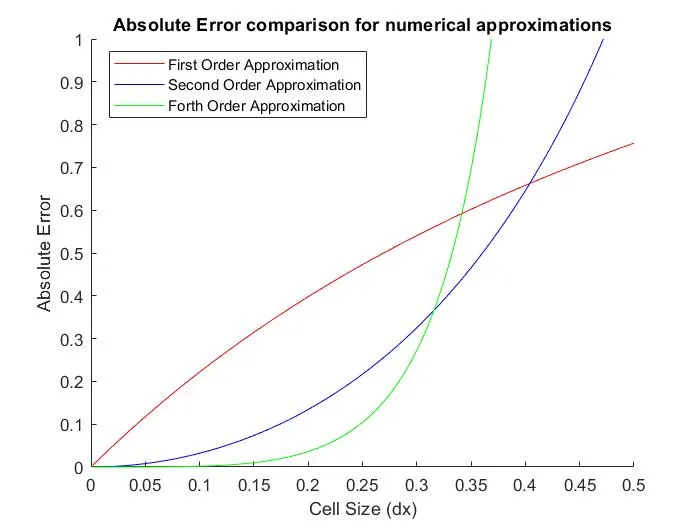
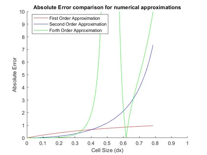
• The error comparison for decreasing calues of dx
• 
• Figure 1 Figure 2

BAR GRAPH:

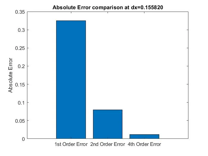
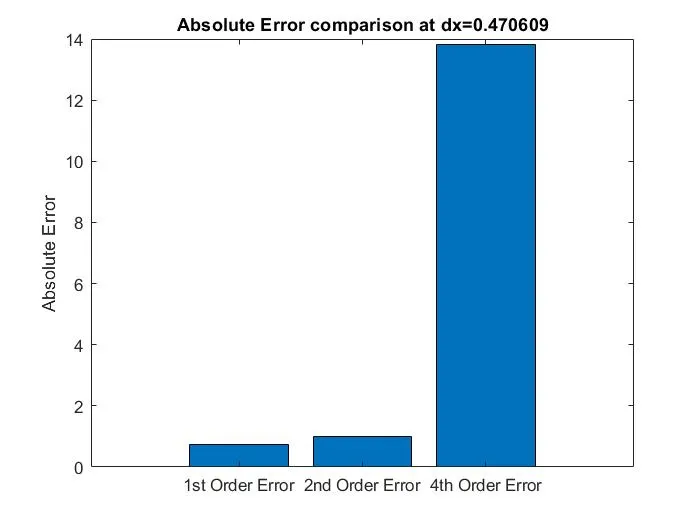
• At dx=0.155820 At dx=0.470609
• 
• Figure 3 Figure 4

CONCLUSION:

• In Figure 1, the real difference is approximations are observed when zoomed into smaller dx values. As the dx values keep decreasing the error value of the forth order approximation reduces exponentially.
• Figure 2 shows a sudden spike in error values of forth order approximation at dx=0.5. This is happeing because of the sin(x) function. When observed the `pi/3` point of interest lies in the positive regime. The computation of first and second order approximations constitute terms such as `f(x+Deltax)` and `f(x-Deltax)` for a value of `Deltax=0.5`. All these function values lie in the positive regime. While computing the forth order approximation of the function derivative, `f(x+2Deltax)` and `f(x−2Deltax)` are used dwhich stretch the stencil to the negative regime either above `x=pi/2` or below `x=0`. The negative value computation with an absolute error calculation is producing a very high error value at the dx value.
• Figure 3 and 4 are a comparison of the absolute error vlaues at different input dx values. At the the lower end, in Figure 3, the forth order approximation is very low. But according to the logic explained in earlier point the error of forth order approximation is Figure 4 is very high near dx=0.5.