Parametric study on Gate Valve in ANSYS Fluent

CFD SIMULATION OF CYCLONE SEPARATOR USING DISCRETE PHASE MODELLING

AIM:

Perform a parametric study on the gate valve simulation by setting the opening from 10 % to 80%.

• Obtain the mass flow rates at the outlet for each design point.
• Calculate the flow coefficient and flow factor for each opening and plot the graph.
• Discuss the results of the mass flow rate and flow coefficient.

INTRODUCTION:

A gate valve is generally used to completely shut off fluid flow or, in the fully open position, provide full flow in a pipeline. Thus it is used either in the fully closed or fully open positions. A gate valve consists of a valve body, seat and disc, a spindle, gland, and a wheel for operating the valve. The seat and the gate together perform the function of shutting off the flow of fluid. Gate valves are generally not suitable for regulating flow or pressure or operating in a partially open condition. For this service, a plug valve or a control valve should be used. It must be noted that because of the type of construction a gate valve requires many turns of the hand wheel to completely open or close the valve. When fully opened, gate valves offer little resistance to flow and its equivalent length to diameter ratio (L/D) is approximately 8.

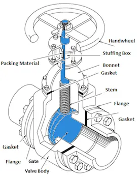
Fig. 1 Gate Valve Schematic

Gate valves work by inserting a rectangular gate or wedge into the path of a flowing fluid. They are operated by a threaded stem which connects the actuator (generally a hand wheel or motor) to the stem of the gate. If the valve has a rising stem its position can be seen just by looking at the position of the stem. One reason that gate valves are not normally used to regulate flow is that the flow rate of the fluid is not proportional to the amount that the valve is open. Moreover, a partially open gate valve may suffer from vibration in which the valve may move from its assigned position. Also the gate and seat may be subject to excessive wear if the valve is partially open.

The Flow Coefficient of a device is a relative measure of its efficiency at allowing fluid flow. It describes the relationship between the pressure across an orifice valve or other assembly and the corresponding flow rate.

`C_v=Qsqrt((SG)/(DeltaP))`

where

`C_v` : Flow Coefficient or flow capacity rating of a valve

`Q` : Flow rate (gallons per minute)

`SG` : Specific Gravity of fluid (water=1)

`DeltaP` : Pressure Drop across the valve (psi)

The metric equivalent of Flow Coefficient is Flow Factor.

`K_v=Qsqrt((SG)/(DeltaP))`

where

`K_v` : Flow Factor or flow capacity rating of a valve

`Q` : Flow rate (`m^3/(hr)`)

`SG` : Specific Gravity of fluid (water=1)

`DeltaP` : Pressure Drop across the valve (bar)

The relationship between `K_v` and `C_v` is:

`K_v=(0.865).C_v`

SOLVING AND MODELLING APPROACH:

The following flow chart is followed for the Solving Approach:

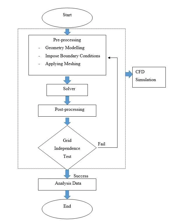
Fig. 4 Solving Approach Flow Chart

ANSYS involves selection of Fluent solver, input and verification of Geometry, Meshing, Setup, Solutions and Results. The Geometry is input in ANSYS Space Claim. The mesh sizing and face naming is done while Meshing. The Setup section involves Mesh Checking, Turbulence Model selection, Solver type, velocity formulation and time (steady or transient state), Output report files, Material selection, Initial and Boundary conditions. The Results section is used for the visualiztion of the output in a GUI.

PRE-PROCESSING AND SOLVER SETTINGS:

GEOMETRY:

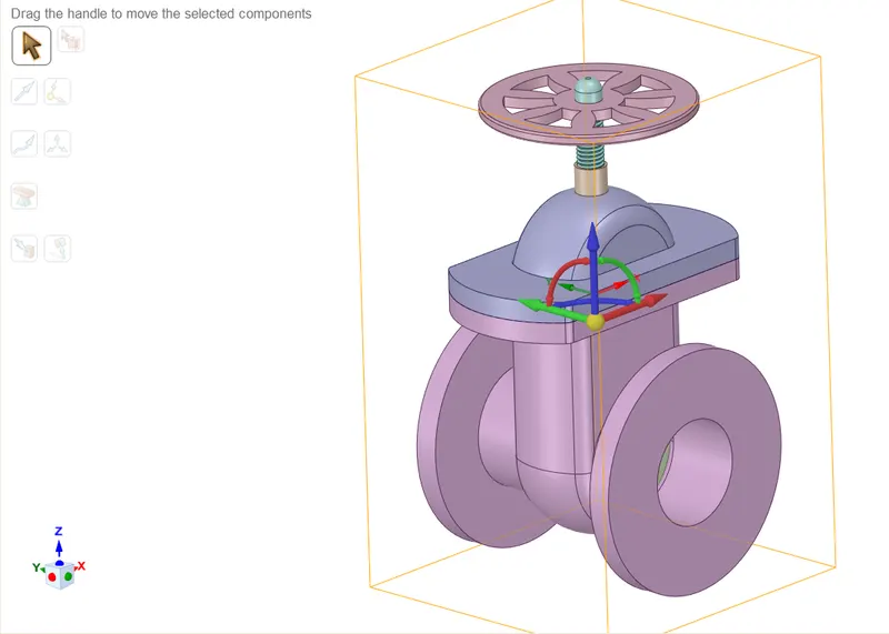
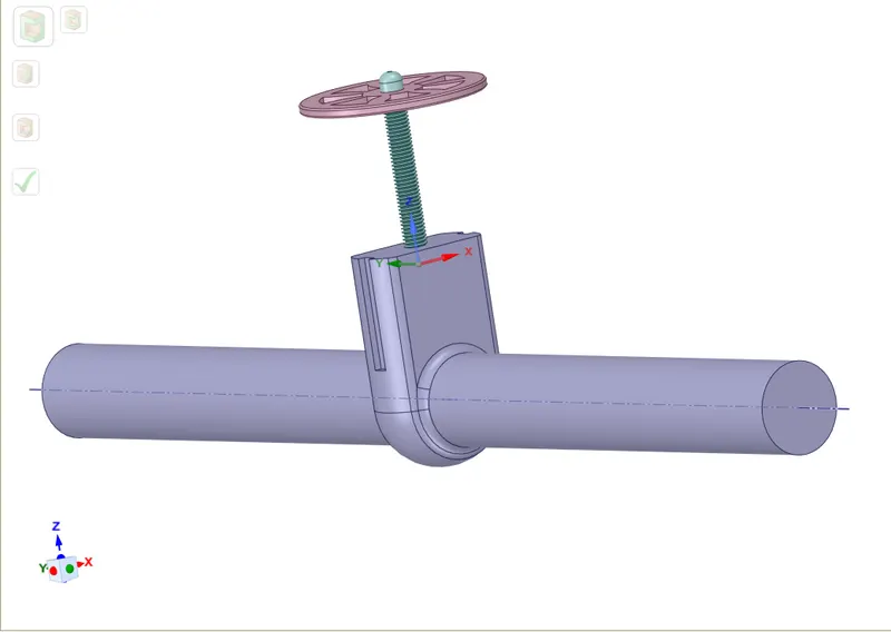
(a) (b)

Fig. 1 (a)CAD Geometry for Gate Valve ,(b) Extracted enclosure geometry

The above geometry is imported into Spaceclaim. Volume extract feature is used to create a volume where the fluid flows. The Gate Valve geometry is Suppressed for Physics to only consider the enclosure for fluid interactions. The Move option was used to move the Disc up in the z-direction. The Parameterize option was used before setting up the displacement moved. This input into Fluent as a varying parameter. The Update Volume Body in context is selected by right-clicking the extracted volume structure on the panel. This ensures that the fluid enclosure created is also updated with the moving Disc. To ensure that every time the Volume Enclosure prepared has a defined inlet and outlet length, the faces of the Bottom structure are extended by 500mm using Pull option.

MESHING:

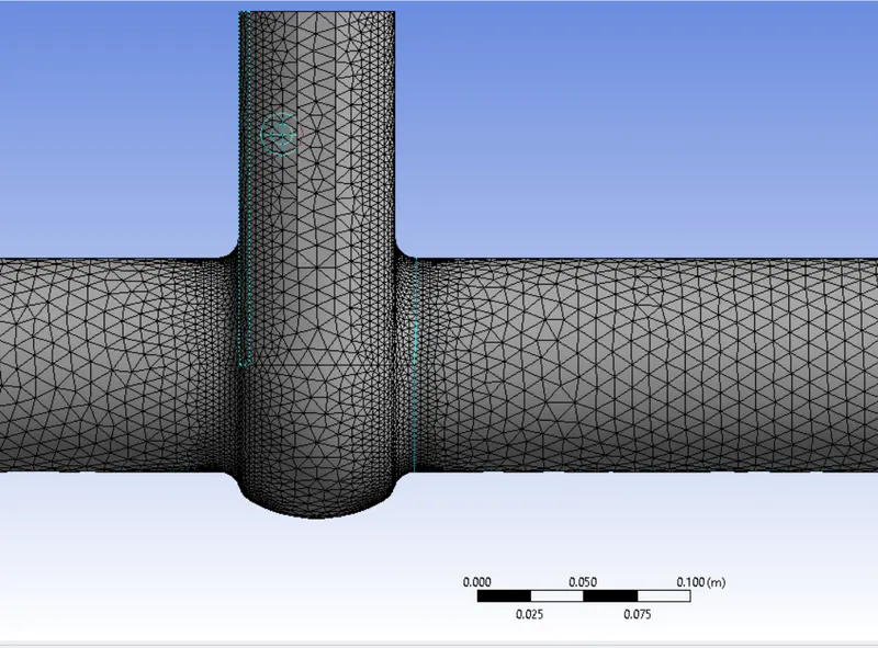
Fig. 2 Meshing for the Geometry

A baseline mesh was created with element size of `1e^(-2)m`. The respective faces were named Inlet and Outlet. The wall condition is automatically taken by Fluent for the un-named faces.

SETUP:

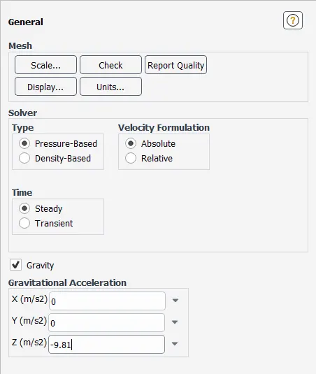
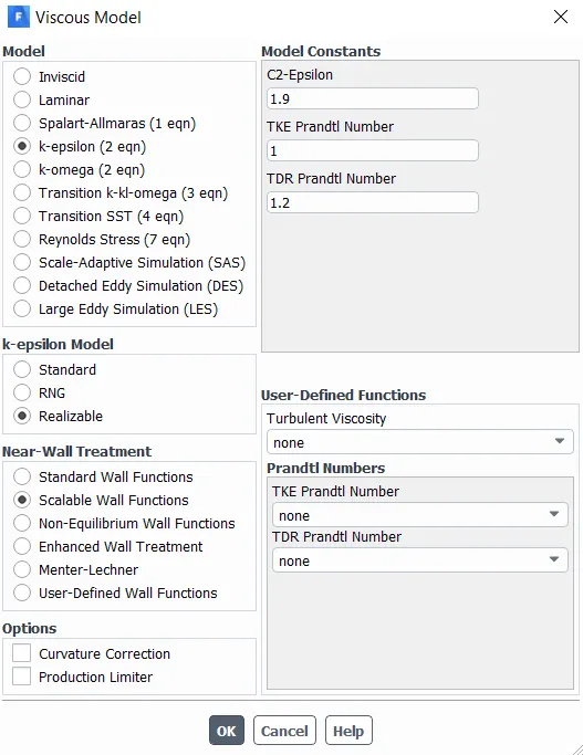
Since the problelm statement is considered for a low Mach number, a Pressure Based Solver is considered for the simulation. The `k-epsilon` Realizable Turbulence model was used for the respective test case calculations. In the model Scalable Wall Functions is activated.

(a) (b)

Fig. 3 (a)Setup- Solver, (b) Setup- Viscous Model

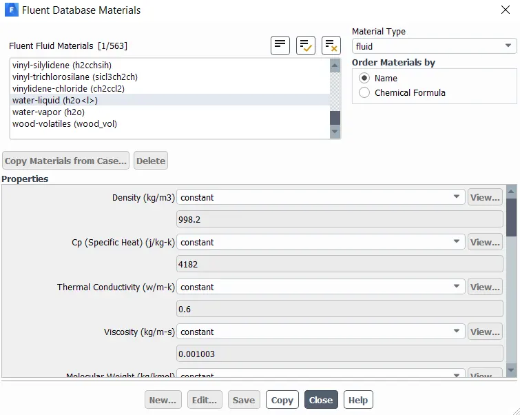
A Steady State simulation is run. In the Physics section, Add Materials option is used to add water (fluid) from the Fluent Database. In Cellzones, the Volume fluid should be changed to water as it is the fluid used for the simulation.

(a)

Fig. 4 Fluent Database Materials

For Boundary Conditions, the Inlet is given a pressure-inlet input with 10Pa. The Outlet is automatically given a gauge pressure of 0Pa.

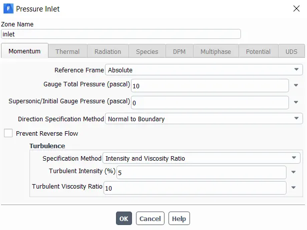
Fig. 5 Boundary Condition Setup example for Inlet Phase

The Standard Initialization is used wherein the user inputs the initial velocity and face from where computation will start (Inlet). In Definitions, New Flux Report is created for Mass Flow Rate at the Outlet face. The Create Output Parameter is used to set this as the output varying dependent on the input parameters.The simulation is run for 500 iterations.

RESULTS:

Table 1: Parametric Study for the input parameters

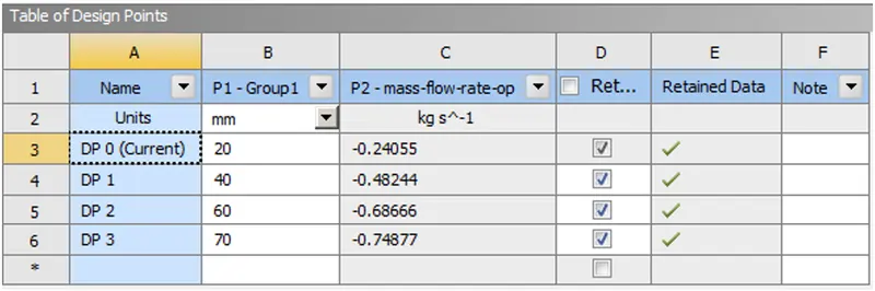
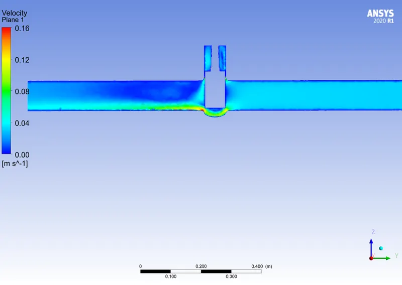
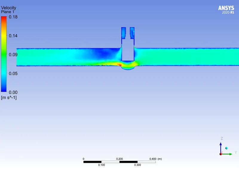
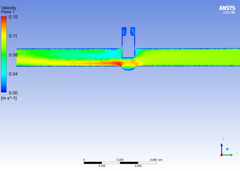
The following velocity and pressure contours were obtained as the input paramter was varied:

Table 2: Differentiating the velocity and pressure contours for the paramteric displacements 20,40,60 and 70 mm.

Parameter Input	Pressure Contour	Velocity Contour
D= 20mm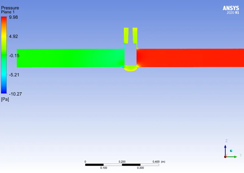
D= 40mm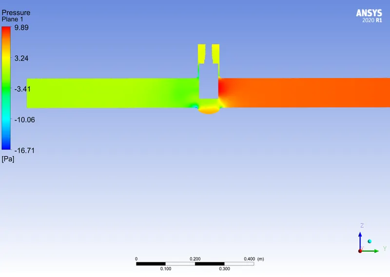
D= 60mm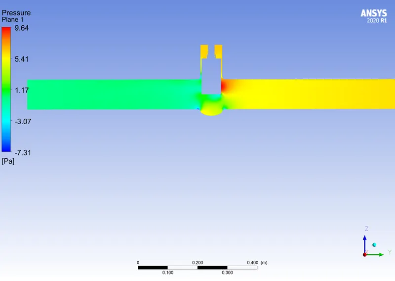
D= 70mm

Table 3: Calculation of Flow Coefficient and Flow Factor

Paramteric Shift	Flow Rate (kg/s)	Volume Flow Rate (`m^3/(hr`)	Pressure Drop (Pa)	Pressure Drop (psi)	Flow Factor (`m^3/(hrtext(bar)^0.5)`)	Flow Coefficient (`(gal)/(mintext( psi^0.5))`)
20 mm	0.24055	0.86858	10.0	`10xxe^(-5)`	86.858	100.414
40 mm	0.48244	1.74201	10.0	`10xxe^(-5)`	174.201	201.388
60 mm	0.68666	2.47941	10.0	`10xxe^(-5)`	247.941	286.636
70 mm	0.74877	2.70368	10.0	`10xxe^(-5)`	270.368	312.564

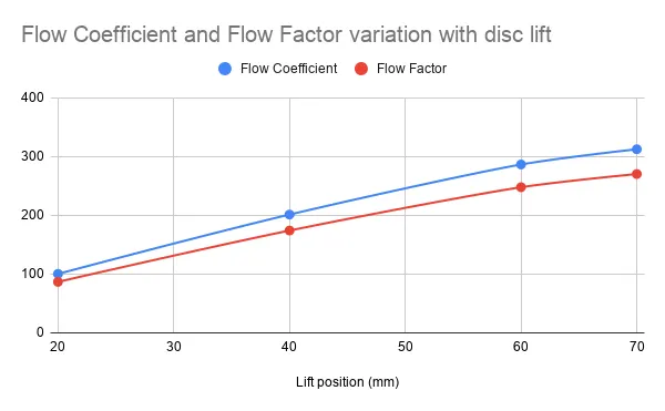
Fig. 6 Graphical Comparison of Flow parameters with the Disc Lift

CONCLUSION:

The use of the flow coefficient offers a standard method of comparing valve capacities and sizing valves for specific applications that is widely accepted by industry.

The flow rate increases as the disc valve displacement increases.

Both the Flow coefficient and Flow factor are directly proportional to the volumetric flow rate, and hence increase with the valve disc displacement increament.

A sudden pressure drop is observed upto 40 mm disc displacement, and at higher displacements a more uniform pressure drop is obtained.