Linear Convection

1D LINEAR CONVECTION

AIM:

• Write a MATLAB code to solve the 1D linear convection equation for number of grid points 20,40,80,160.

OBJECTIVES OF THE PROJECT:

• Solve the 1D linear convection equation for a first order forward differencing in time and first order backward differencing in space.
• Reach the final solution at specified time and plot velocity profile for each case.

GOVERNING EQUATIONS:

• The 1D linear convection equation is stated as:
• `(delu)/(delt)+c(delu)/(delx)=0`_____(1)
• Where `c` stands for the speed of the wave and `u` stands for the velocity.
• The individual derivatives when broken into respective first order numerical approximations:
• First order forward differencing in time
  `(delu)/(delt)=(u_i^(n+1)−u_i^n)/(Deltat)`_____(2)
• First order backward differencing in space
• `(delu)/(delx)=(u_i^n−u_(i−1)^n)/(Deltax)`_____(3)
• Substituting Eqn.2 and 3 in 1:
• `(u_i^(n+1)−u_i^n)/(Deltat)+c(u_i^n−u_(i-1)^n)/(Deltax)=0`
• Therefore,
• `u_i^(n+1)=u_i^n-(cDeltat)(u_i^n−u_(i-1)^n)/(Deltax)`_____(4)
• Eqn 4 is used for each time step n">nn and each grid point i">ii in the computation of the final velocity profile.

BODY OF THE CONTENT:

• CODE:

• clear all,close all,clc
  %1D Linear Convection
  %Input parameters for the flow
  %Length of domain
  L=1;%units=m
  %Number of nodes
  n=80;
  %speed of wave
  c=1;%units=m/s
  %dt is the time step selected
  dt=0.01;%units=m
  
  %Calculations
  %domain is divided into n nodes
  x=linspace(0,L,n);
  %The cell size is calculated
  dx=x(2)-x(1);
  
  %Apply Boundary Conditions
  %Except for 0.1<x<0.3, all="" the="" nodes="" in="" domain="" have="" 1m="" s="" velocity="" u="ones(1,n);" %a="" loop="" is="" run="" to="" assign="" 0.1<x<0.3,="" a="" 2m="" veloctiy="" profile="" for="" i="1:length(x)" if(x(i)="">=0.1 && x(i)<=0.3)
     u(i)=2;    
     end     
  end   
  %The initial velocity profile is captured in two variables, one for final
  %comparison and other as initial condition for the calculation of the next
  %time step velocity value
  uold=u;
  uoriginal=u;
  %Time Marching Solution
  %The problem statement describes a velocity profile upto 0.4s. Therefore, a
  %quantity nt is described. nt is the number of times the loop will run.
  %therefore nt*dt=40*0.01=0.4s. The solution upto desired time is calculated
  nt=40;
  for k=1:nt
     for i=2:n
         %forward differecing in time, as the uold (previous data set) is
         %used. Backward diffencing in space, as uold(i) and uold(i-1) are
         %used in the space derivative
        u(i)=uold(i)-(c*dt/dx)*(uold(i)-uold(i-1)); 
     end   
     % The above loop was run for one time frame and all the nodes. Yhe
     % solution obtained for this time step is updated as uold, for
     % calculation of the next time step in next loop
     uold=u;
  end    
  
  %Plotting of initial and final velocity profiles
  plot(x,uoriginal,'b','linewidth',1.5)
  hold on
  plot(x,u,'r','linewidth',1.5)
  axis([0 1 0 3])
  grid on
  legend('Initial Velocity','Final Velocity')
  title('1D Linear Convection Velocity Profile')
  xlabel('Length (m)')
  ylabel('Velocity (m/s)')</x<0.3,>

• Explanation: The constant input parameters such as domain length (`L`), number of nodes in domain (`n`), speed of wave (`c`) and time step (`dt`) are specified. The domain is divided based on the number of nodes and the cell size `dx` is found out. The initial conditions for the velocity profile is input wherein a loop is run over x vector and all the points in the domain 0.1<x<0.3 . As the velocity profile is known for t=0, it is apploed in Eqn.4 for the next time frame. This is done in a loop for each time frame, till the velocity profile for t=0.4s is reached. Another loop inside this loop is run for computation of velocity profile based on Eqn.4 for each node on the grid. After this loop finished the uold">uold profile is updated to the current u">uu profile. This is done because for the next time step, the `u_i^n` velocity vector would be the current computed velocity profile. Once the final profile at t=0.4s is computed, the original and final profiles are plotted for each test case.
• OUTPUT:
• For n=20: For n=40:
• 
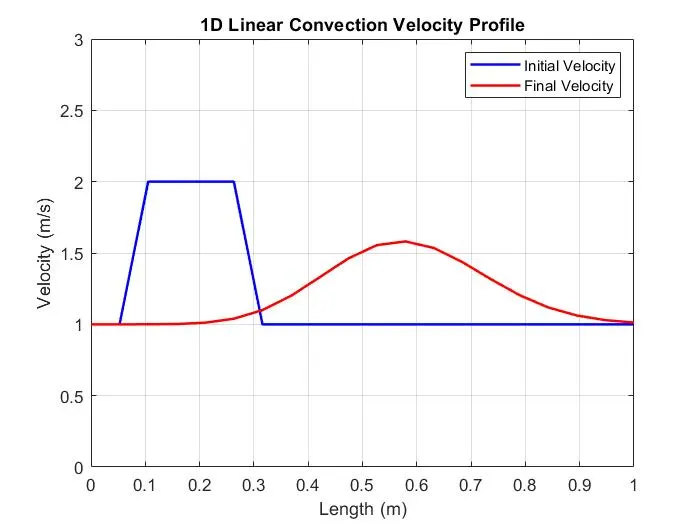
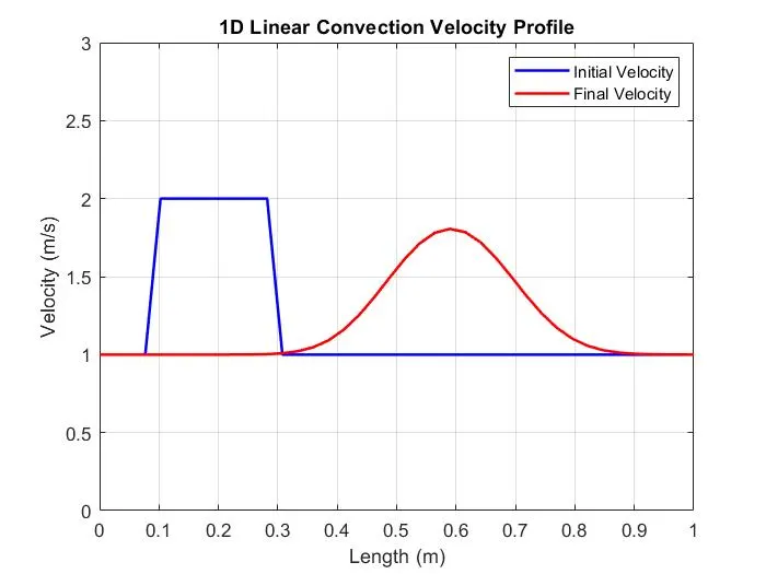
• For n=80: For n=160:
• 
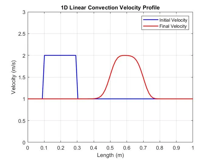
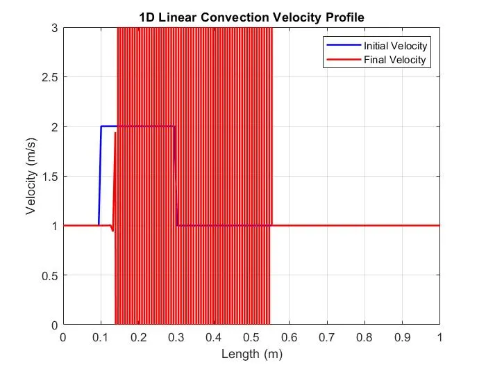
• It can be observed in each figure that the curve smoothens as the number of grid points are increased. But in the n=160 domain, a large blowup is observed.

CONCLUSION:

• The figures show better smoothness and retentioon of the velocity profile. The velocity dropped down faster in n=20 profile because the artificial diffusion terms are ignored. the diffusion terms are comprised of the second order derivatives of velocity, which are not considered in this analysis. The difference in the peak velocity is basically the error terms in the second order form of diffusion.
• The increase in the velocity in the n=40 and 80 plot is obseved because of larger number of grid points. Larger number of grid points are improving the accuracy by computing closer solutions to the actual convection profile. When `Deltax` gets smaller with more number of grid points, the error terms or the diffusive terms also get smaller and the peak velocity reaches closer to peak velocity.
• The last figure for n=160, clearly shows that the solution is blowing up. This unstability is observed because of Gibb's Phenomenon. This phenomenon explains that while using a numerical approximation to define the discontinuous points in a function, overshoots are observed. these overshoots are finite in nature and can be resolved by adding more terms to reduce the error developed in the velocity field, i.e. increasing the order of the numerical approximation.