CFD Simulation for flow over an Ahmed Body using ANSYS Fluent
SIMULATION OF AHMED BODY
AIM:
Run a simulation on Ahmed Body to visualize the flow dynamics
Describe Ahmed's body and its importance.
Explain the reason for the negative pressure in the wake region.
Explain the significance of the point of separation.
INTRODUCTION:
Q:Describe Ahmed's body and its importance.
A:
The Ahmed body represents a simplified, ground vehicle geometry of a bluff body type. Its shape is simple enough to allow for accurate flow simulation but retains some important practical features relevant to automobile bodies. This model describes how to calculate the turbulent flow field around a simple car-like geometry using the Turbulent Flow, k-epsilon interface. The simulation is used for optimizing external aerodynamics of an automotive. The simulation gives a clear visualization on the pressure distribution, velocity and turbulent properties over the Ahmed Body for various Reynolds Numbers. The location at which the flow separates determines the size of the separation zone, and consequently the drag force. Clearly, a more exact simulation of the wake flow and of the separation process are essential for the correctness of drag predictions. The flow separation varies for the slant angle `phi`, and this is a major contributing factor for the simulation analysis.
GEOMETRY:
The geometry is created based on the simplified aerodynamic body used by Ahmed et al. See Fig.1. for dimensions. The slant angle (`phi`) is set to 25 degrees. The body is placed in a wind tunnel (8m×1.4m×1.3m) in order to limit the aerodynamic blockage effect.
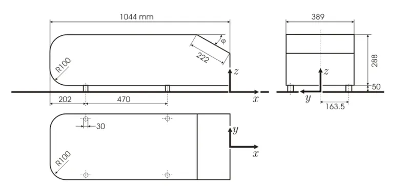
Fig. 1 Dimensions of the Ahmed Body
Q:Explain the reason for the negative pressure in the wake region.
A:
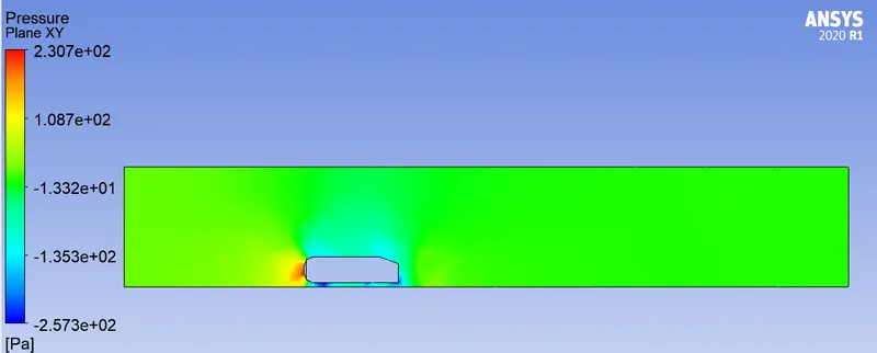
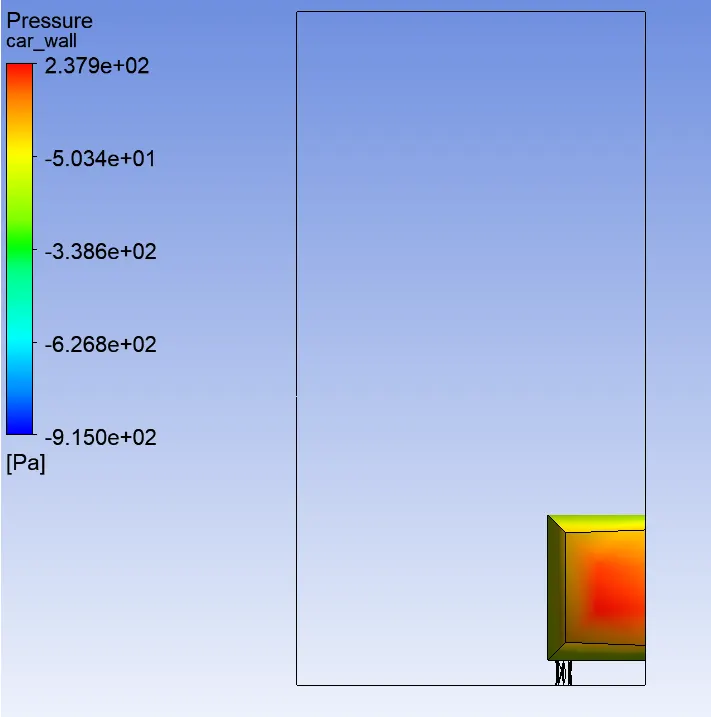
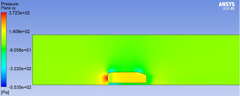
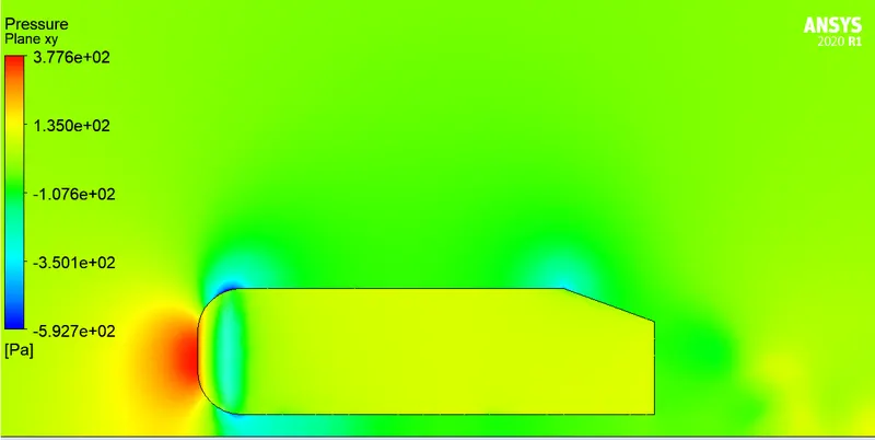
The problem statement is solved for a Reynolds Number: `Re=(rhovD)/mu=(25.(1.044))/(1.56e^(-5))=1.67e^6`. Therefore the flow is in turbulent state. In turbulent flow, the flow develops to separated state. A high pressure region is created right in front of the body as the air is pushed up into the mainstream, and similarly an adverse drop is observed when the flow detaches at the slant angle behind the Ahmed Body. This detachement or separation of flow leads to eddy formation and disturbance in the flow. The viscous effects of the fluid are only restricted to the boundary layer till the flow is attached and there is an increase in the boundary layer width as the flow shifts into turbulent zone (separated). The boundary layer thickness increases and becomes unstable. This region behind the Ahmed body where the flow is unstable is termed as Wake, where the pressure adversely drops. Because of viscous losses, the stagnation pressure in the wake is lower than the stagnation pressure at the front of the body. This shows a negative pressure region in the Wake Zone. For a drop in angle at the rear end (after the slant edge), the pressure force and the force due to streamwise acceleration i.e. inertia forces are acting in the same direction creating this negative pressure gradient.
It has been observed that across the boundary layer the pressure remains constant. This means that the streamwise pressure gradient in the boundary layer is the same as the pressure gradient along the wall in the outer (inviscid) flow i.e., the external pressure is ‘impressed’ upon the boundary layer. Therefore, the flow within the boundary layer is subjected to a decreasing pressure (negative gradient).
Q:Explain the significance of the point of separation.
A:
It has been observed that the flow is reversed at the vicinity of the wall under certain conditions. The phenomenon is termed as separation of boundary layer. Separation takes place due to excessive momentum loss near the wall in a boundary layer trying to move downstream against increasing pressure, i.e., `(delp)/(delx)>0` , which is called adverse pressure gradient.
Fig. 2 Flow separation and formation of wake behind a circular cylinder
So long as no viscous effect is considered, the situation does not cause any sensation. In the viscid region (near the solid boundary), Up to , the viscous force opposes the combined pressure force and the force due to acceleration. Fluid particles overcome this viscous resistance due to continuous conversion of pressure force into kinetic energy. Beyond , within the viscous zone, the flow structure becomes different. It is seen that the force due to acceleration is opposed by both the viscous force and pressure force.
Depending upon the magnitude of adverse pressure gradient, somewhere around , the fluid particles, in the boundary layer are separated from the wall and driven in the upstream direction. However, the far field external stream pushes back these separated layers together with it and develops a broad pulsating wake behind the cylinder. The mathematical explanation of flow-separation : The point of separation may be defined as the limit between forward and reverse flow in the layer very close to the wall, i.e., at the point of separation
This means that the shear stress at the wall, `tau_w=0` . But at this point, the adverse pressure continues to exist and at the downstream of this point the flow acts in a reverse direction resulting in a back flow. It can also explain flow separation using the argument about the second derivative of velocity u at the wall. From the dimensional form of the momentum at the wall, where u = v = 0,
- Consider the case of adverse pressure gradient, `(delp)/(delx)>0`
- At the boundary, the curvature of the profile must be positive (since `(delp)/(delx)>0` ).
- Near the interface of boundary layer and free stream the previous argument regarding and still holds good and the curvature is negative.
- Thus it is observed that for an adverse pressure gradient, there must exist a point for which `(del^2u)/(dely^2)=0` . This point is known as point of inflection of the velocity profile in the boundary layer.
- However, point of separation means `(delu)/(dely)=0` at the wall.
- `(del^2u)/(dely^2)>0` at the wall since separation can only occur due to adverse pressure gradient. But we have already seen that at the edge of the boundary layer, `(del^2u)/(dely^2)<0` . It is therefore, clear that if there is a point of separation, there must exist a point of inflection in the velocity profile.
GOVERNING EQUATIONS AND THEORY:
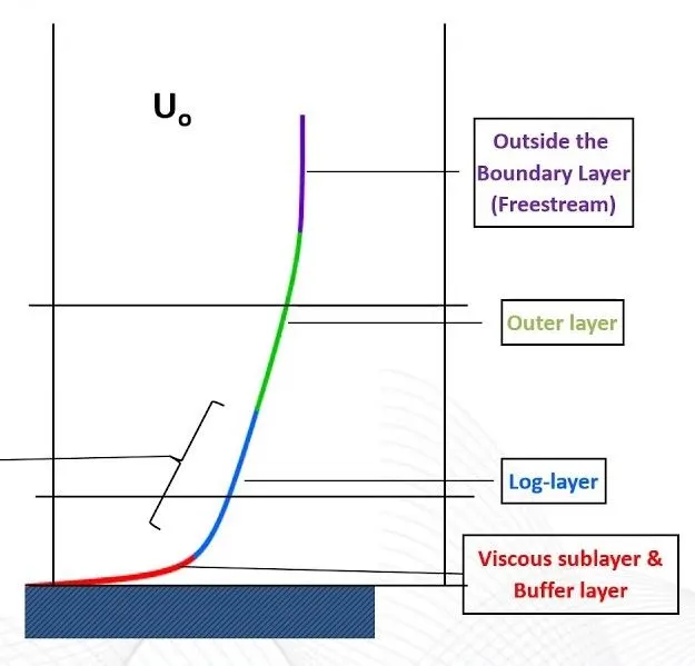
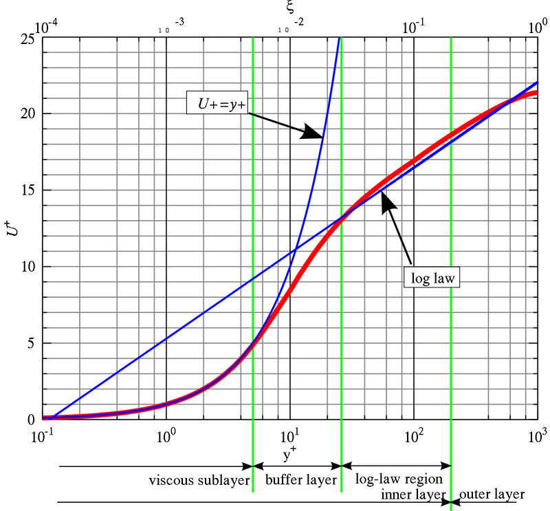
A typical property of the generated mesh is the `y^+` (“y-plus“) value, which is defined as the non-dimensionalized distance to the wall; it is given by
`y^+=(u_t∗y)/ν`. A `y^+` value of 1 would correspond to the upper limit of the laminar sub-layer.
- Full Resolution in the near-wall region: The first cell lies at most at the boundary of the laminar sub-layer and no further. Here, `y^+` value is 1 or below.
- Use of wall-functions to resolve the near-wall region: There is no need to place cells very close to the laminar sub-layer, and typically `30<=y^+<=300`.
(a) (b)
Fig. 3 (a) Turbulent Boundary Layers (b) Law of the Wall
`k-epsi` turbulence model only resolves the boundary layer in the log-layer, so requires a `y^+` between 20 and 100. If `y^+` is too high, the mesh is under resolved and the mesh should be refined normal to the wall.
`text(SST k-omega)` resolves the boundary layer in the viscous sub-layer. A `y^+~1` for closure is needed to take advantage of this resolution. If `y^+>20` the `k-omega` part of the SST model is not used and simply reduces to `k-epsi` model.
SOLVING AND MODELLING APPROACH:
The following flow chart is followed for the Solving Approach:
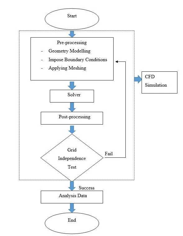
Fig. 4 Solving Approach Flow Chart
ANSYS involves selection of Fluent solver, input and verification of Geometry, Meshing, Setup, Solutions and Results. The Geometry is input in ANSYS Space Claim. The mesh sizing and face naming is done while Meshing. The Setup section involves Mesh Checking, Turbulence Model selection, Solver type, velocity formulation and time (steady or transient state), Output report files, Material selection, Initial and Boundary conditions. The Results section is used for the visualiztion of the output in a GUI.
GRID INDEPENDENCE TEST:
A CFD solution can never be trusted unless it is checked whether the results depend on the grid or not (or through experimental data). The output result of a coarser and finer mesh can never be the same. Grid Independence refers to the mesh setup where the element sizing does not affect the output.This is done by varying the mesh from coarse to fine and checking the output result for each case. When a mesh size is reached where the results are not varying much, the solution is acceptable.
PRE-PROCESSING AND SOLVER SETTINGS:
The input conditions involve inlet flow velocity of `u_0=25text( m/s)`.
GEOMETRY:
The Geometry was input by a pre-defined STEP file. Since the calculation involved flow simulation body to be defined, the Ahmed Body is to be hidden and an enclosure is placed as a wind tunnel as follows:
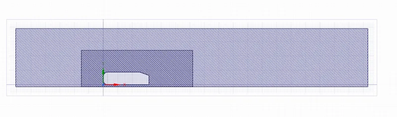
Fig. 5 Enclosure Cut-Section view for Ahmed Body eperiment
An addition enclosure as shown in the figure is introduced for improved cases of simulation to refine the mesh near the wake region of the flow.
MESHING:
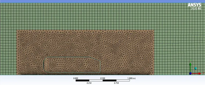
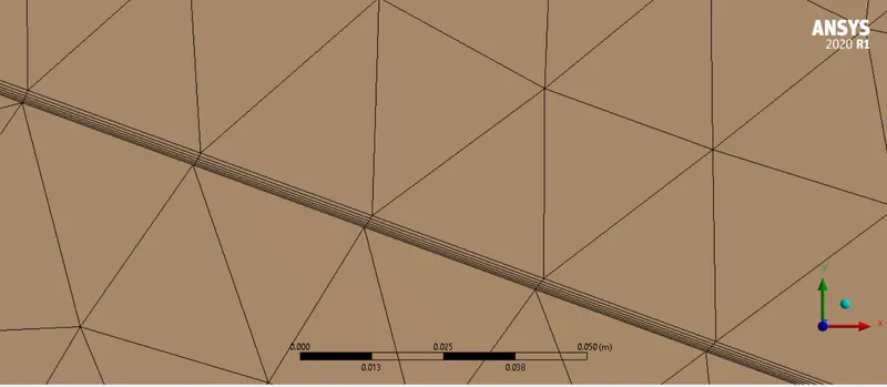
Three Mesh types were examined for the grid independency test. The first case being a single enclosure with element sizes of 0.2m. The second case introducing a second refined enclosure with an element size of 0.05m and hexahedral meshing in the outer enclosure. The third test case includes 6 inflation layers of total thickness 0.0007m and a refined inner enclosure mesh of 0.03m element size. The forth test case includes inner enclosure refinement upto 0.018m and the inflation layer refinement upto 0.0001m. The final case Mesh setup is shown below:
(a) (b)
Fig. 6 (a) Refined Mesh Setup (b) Inflation Layer on the Ahmed Body
It should be noted that Share Topology setup for the FFF Design should be set to SHARE, or the transfer of information among the two enclosures will be restricted and Fluent will consider its own Boundary conditions for the new faces.
SETUP:
Since the problelm statement is considered for a Mach<0.3, a Pressure Based Solver is considered for the simulation. The `k-epsilon` Realizable and `k-omega` SST Turbulence models were used for the respective test case calculations. A plot for drag and lift coefficient and Wall `y^+` value over Ahmed Body wall is plotted against number of iterations. A Steady State simulation is run. The Boundary condition for the Inlet (Velocity=25 m/s), Outlet (Static Pressure= 1 atm) and Symmetry boundary condition for the wind tunnel walls are input. The Ahmed Body is given wall (No slip condition). Hybrid Initialization is used for t=0 and 500 iterations were run for each case.
RESULTS:
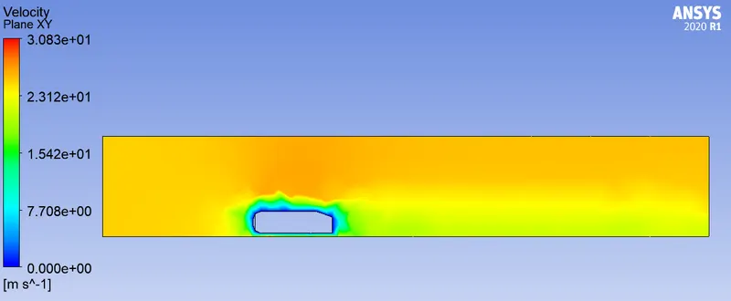
Case 1: Baseline mesh with single enclosure
(a) (b)
(c) (d)
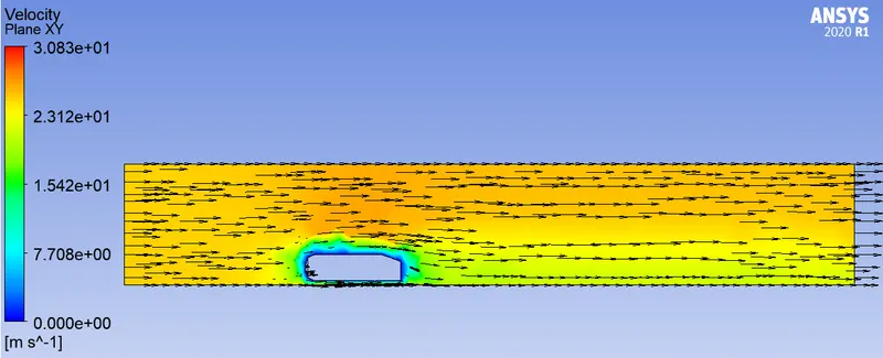
Fig. 7 (a) Velocity profile on plane XY (b) Pressure profile on plane XY (c) Pressure profile on Ahmed Body (Front View) (d) Velocity vector profile on plane XY
Case 2: Medium mesh with double enclosure
(a) (b)
(c) (d)
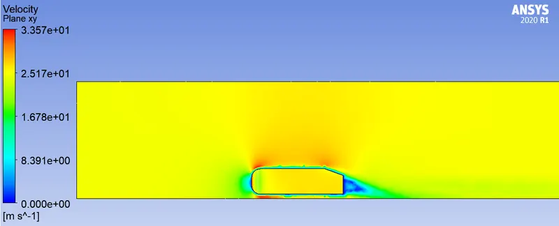
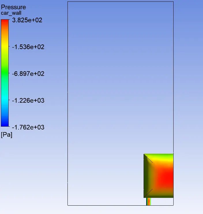
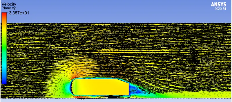
Fig. 8 (a) Velocity profile on plane XY (b) Pressure profile on plane XY (c) Pressure profile on Ahmed Body (Front View) (d) Velocity vector profile on plane XY
Case 3: Refined Mesh with Inflation Layers
(a) (b)
(c) (d)
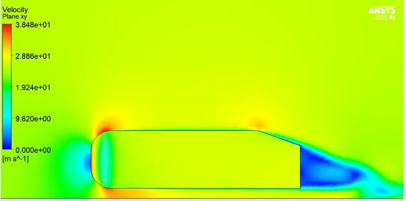
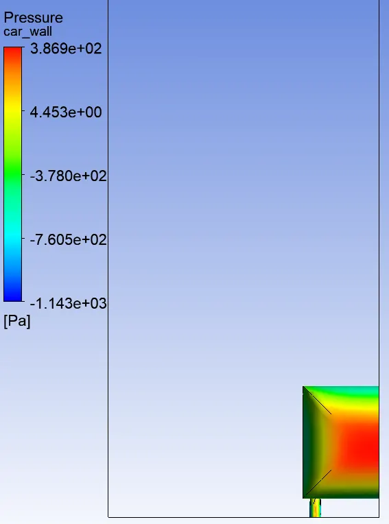
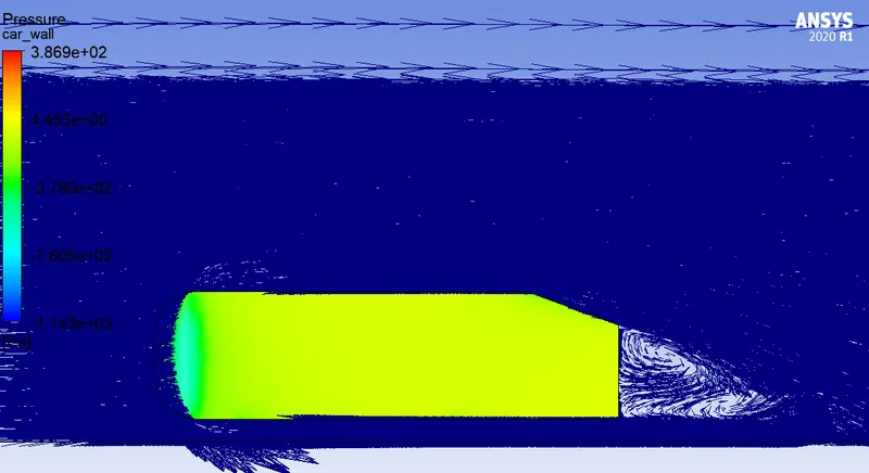
Fig. 9 (a) Velocity profile on plane XY (b) Pressure profile on plane XY (c) Pressure profile on Ahmed Body (Front View) (d) Velocity vector profile on plane XY
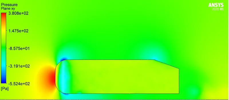
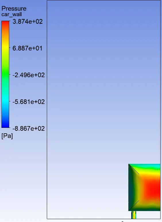
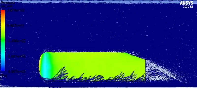
Case 4: Refined Mesh with Inflation Layers (`k-omega` Turbulence Model)
(a) (b)
(c) (d)
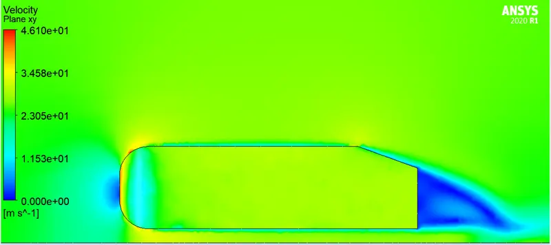
Fig. 10 (a) Velocity profile on plane XY (b) Pressure profile on plane XY (c) Pressure profile on Ahmed Body (Front View) (d) Velocity vector profile on plane XY
A Tabulated result of all the cases:
| `y^+ value` | Lift Force (N) | Drag Force (N) | `C_l` | `C_d` | Outer Enclosure Element Size (m) | Inner Enclosure Elemenet Size (m) | Inflation Layer thickness (1st Layer) (m) | |
| Baseline Mesh without Inner Enclosure | 822.36 | 7.52 | 15.33 | 0.08 | 0.80 | 0.2 | - | - |
| Medium Mesh with Inner Enclosure | 232.28 | 6.67 | 8.43 | 0.35 | 0.44 | 0.05 | 0.03 | - |
|
Refined Mesh with Inflation Layer `k-epsi` |
23.01 | 5.71 | 7.48 | 0.27 | 0.35 | 0.1 | 0.02 | 0.0007 |
|
Refined Mesh with Inflation Layer `k-omega` |
3.08 | 0.85 | 7.39 | 0.04 | 0.34 | 0.1 | 0.018 | 0.0001 |
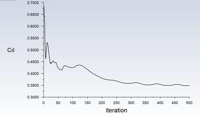
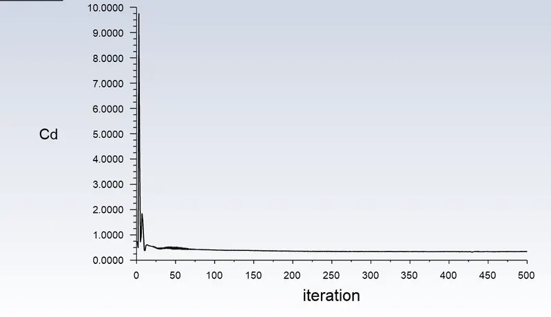
Comparison of Drag coefficient for Case 3 and Case 4 over iterations:
(a) (b)
Fig. 11 (a) Drag coefficient variation for k-epsilon turbulence model (b) Drag coefficient variation for k-omega turbulence model
CONCLUSION:
Stability in the `k-omega` turbulence model simulation was reached earlier and maintained throughout the simulation.
As the mesh grew finer, and the region including the wake was refined, the drag coefficient and `y^+` values were reaching rhe theoretical values.
The negative pressure in the wake region behind the Ahmed Body is a result of dominance of pressure and viscous forces over the accelearating force of fluid. Pressure in the wake remains close to separation-point-pressure since the eddies cannot convert rotational kinetic energy into pressure head. The wake zone pressure is less than that of the forward stagnation point, the Ahmed Body experiences a drag force which is basically attributed to the pressure difference.
The close examination of vector fields in the wake region show a circulation of the flow due to the Flow Separation.