CFD Simulation capturing Gearbox Sloshing Effect in ANSYS Fluent

GEARBOX SLOSHING EFFECT

AIM:

Perform four simulations in the Gearbox and then compare the results among all the four cases.

1. 20% Immersion, Fluid - Engine oil.
2. 30% Immersion, Fluid- Engine oil.
3. 20% Immersion,Fluid-n-heptane (c7h16).
4. 30% Immersion,Fluid-n-heptane (c7h16).

INTRODUCTION:

Q:What is Dynamic meshing? Give some other examples where dynamic meshing can be used.

A:

Dynamic Meshing allows the user to move the boundaries of a cell zone relative to other boundaries of the zone. The motion can be linear, rotational or deformative. Dynamic Meshing is applied when the nodes defining the cells are updated as a function of time, i.e. unsteady deformations. This type of meshing requires initial description of the moving, non-moving and deforming zones. The Dynamic Meshing in ANSYS Fluent is divided into three types- Smoothing, Dynamic Layering and Remeshing Methods. Each method has a different set of criterias, which need to be satisfied for use in problem solving of that case. Sliding Mesh is a subset of Dynamic Meshing wherein the cells of a mesh zone move together in a rigid-body motion and include no deformation One advantage of this case is that the mesh zones defining the respective motions need not be conformal interfaces.

An example of linear translation where a ball is dropped from one fluid (air) into the other fluid (water). An example of rotational translation can be analysis of fluid motion in a centrifugal pump due to the action of the rotor blades.

Q: What is the fluid Sloshing effect? Discuss whether the sloshing effect is good or bad? Explain.

A:

Sloshing means any motion of the free liquid surface inside its container. It is caused by any disturbance to partially filled liquid containers. Depending on the type of disturbance and container shape, the free liquid surface can experience different types of motion including simple planar, nonplanar, rotational, irregular beating, symmetric, asymmetric, quasi-periodic and chaotic. Under low gravity fields, the surface tension is dominant and the liquid may be oriented randomly within the tank depending essentially upon the wetting characteristics of the tank wall. The basic problem of liquid sloshing involves the estimation of hydrodynamic pressure distribution, forces, moments and natural frequencies of the free-liquid surface. These parameters have a direct effect on the dynamic stability and performance of moving containers.

Unfavourable sloshing occurs in examples such as Oil Tanker transportation. One disadvantage of such sloshing is the sudden momentum transfer due to sloshing, as the internal pressure distribution affects the tank’s motion. In such cases, additional intermediate porous walls are added, to reduce the sloshing effect. Each section of the tank is filled with different proportions of the oil to maintain the centre of gravity close to the truck’s head; this gives more control to the driver.

Sloshing is useful in situations such as hydrokinetic energy, when energy is extracted from the tidal waves of the ocean. When a container carrying a magnetized ferrofluid is subjected to external mechanical stimuli, the sloshing motion of the magnetized ferrofluid generates a time-varying magnetic flux, which can be used to induce an electromotive force in a coil placed adjacent to the container. This process generates an electric current in the coil, and therewith, can be used to transduce external vibrations into electrical energy.

Q: What is the use of UDF?

A:

UDFs allow you to customize Fluent to fit your particular modeling needs. UDFs can be used for a variety of applications. Some examples include

• customization of boundary conditions , material property definitions, surface and volume reaction rates , source terms in transport equations, source terms in user-defined scalar (UDS) transport equations , diffusivity functions , etc.
• adjustment of computed values on a once-per-iteration basis
• initialization of a solution
• asynchronous (on demand) execution of a UDF
• execution at the end of an iteration, upon exit from Fluent, or upon loading of a compiled UDF library
• Post processing enhancement
• enhancement of existing Fluent models (e.g., discrete phase model, multiphase mixture model, discrete ordinates radiation model)

Q: Discuss the common errors that occurred in the simulation. (a) 'Dynamic mesh failed' error. (b) 'Negative cell volume detected' error.

A:

(a)

Update Dynamic Mesh failed refers to problems observed during the dynamic mesh distortion. The input user defined functions and the marked regions create the respective motion desired. This requires a change in meshing which is being adhered. Large mesh element sizes can affect the local solution as each time step has a new mesh orientation. Dynamic Meshing can be refined using Remeshing and Smoothing methods.

(b)

This error means that the element has a big distortion. Big enough to do some vertex, or edges, to penetrate an opposite face resulting in a negative volume, once it is calculated based on the metrics and the local coordinate system of the element that represents the volume of control. A negative volume will generate unphysical behavior of equations. The time step is probably large when compared with the displacement of your mesh. A good practice is to limit the displacement to 1/2 length scale of the adjacent volumes from the moving boundary. You will reach that decreasing your time step.

SOLVING AND MODELLING APPROACH:

The following flow chart is followed for the Solving Approach:

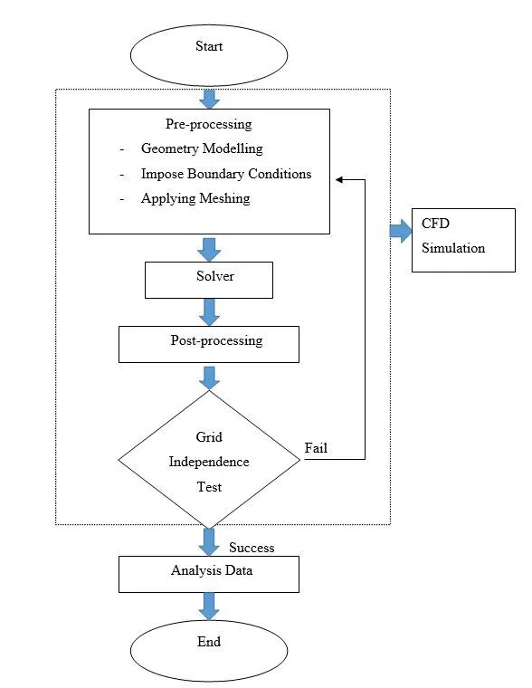
Fig. 4 Solving Approach Flow Chart

ANSYS involves selection of Fluent solver, input and verification of Geometry, Meshing, Setup, Solutions and Results. The Geometry is input in ANSYS Space Claim. The mesh sizing and face naming is done while Meshing. The Setup section involves Mesh Checking, Turbulence Model selection, Solver type, velocity formulation and time (steady or transient state), Output report files, Material selection, Initial and Boundary conditions. The Results section is used for the visualiztion of the output in a GUI.

PRE-PROCESSING AND SOLVER SETTINGS:

GEOMETRY:

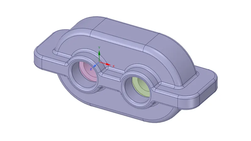
Fig. 1 CAD Geometry for Gearbox

The above geometry is imported into Spaceclaim. Volume extract feature is used to create a volume where the fluid flows. The body is split into 2 using the split body command and the XY Plane. The face of the enclosure created is copied and saved in another file. This geometrical setup is used as a 2D simulation is run.

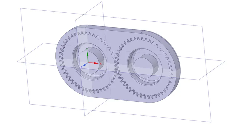
Fig 2. Split Body of volume extracted

MESHING:

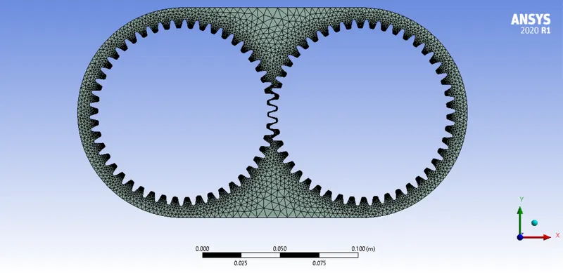
Fig. 3 Meshing for the Geometry

A baseline mesh was created with element size of 14.2 mm. The respective faces were named left gear and right gear. Method option in Insert was used to create a Triangular Meshing Method. The Capture Proximity option was enabled in the Mesh Sizing option. Number of cells across the gap was set to 3.

SETUP:

Since the problelm statement is considered for a low Mach number, a Pressure Based Solver is considered for the simulation. The `k-epsilon` Realizable Turbulence model was used for the respective test case calculations. A Transient State simulation is run. In the Models section, Multiphase- Volume of Fluids option is enabled. Implicit solving method is used. Gravity option is enabled and the value is set to 9.81 in the Y direction. In Setting Up Domain, the Mark/Adapt Cells option was enabled and a Quadrilateral region was created to mark the cells (Inside).

20% Immersed:

`(X_min,Y_min)=(-0.0675,-0.0675)`

`(X_max,Y_max)=(0.1825,-0.0405)`

30% Immersed:

`(X_min,Y_min)=(-0.0675,-0.0675)`

`(X_max,Y_max)=(0.1825,-0.0270)`

In User Defined, Functions is enabled using Compiled option. The following file is Added, Built and Loaded.

#include "udf.h"

DEFINE_CG_MOTION(right_motion, dt, vel, omega, time, dtime)
{
	vel[0] = 0.0;
	vel[1] = 0.0;
	vel[2] = 0.0;

	omega[0] = 0.0;
	omega[1] = 0.0;
	omega[2] = 2.0e2; /* [rad/s]*/
}
DEFINE_CG_MOTION(left_motion, dt, vel, omega, time, dtime)
{
	vel[0] = 0.0;
	vel[1] = 0.0;
	vel[2] = 0.0;

	omega[0] = 0.0;
	omega[1] = 0.0;
	omega[2] = -2.0e2; /* [rad/s]*/
}

In Setting Up Domain, Dynamic Meshing is enabled and the Left Motion was enabled for the Left Gear at (0,0) and Right Motion for the Right Gear at (0.115,0)(metres). Hybrid Initialization was used for t=0 condition. The Patch option was enabled, where the respective fluid was selected and Volume Fraction optiion was used to Patch the region with value 1. The respective materials were selcted from the Fluent Base and added as Secondary Phase in the Phases option in Multiphase.

RESULTS:

20% Immersion, Fluid - Engine oil:

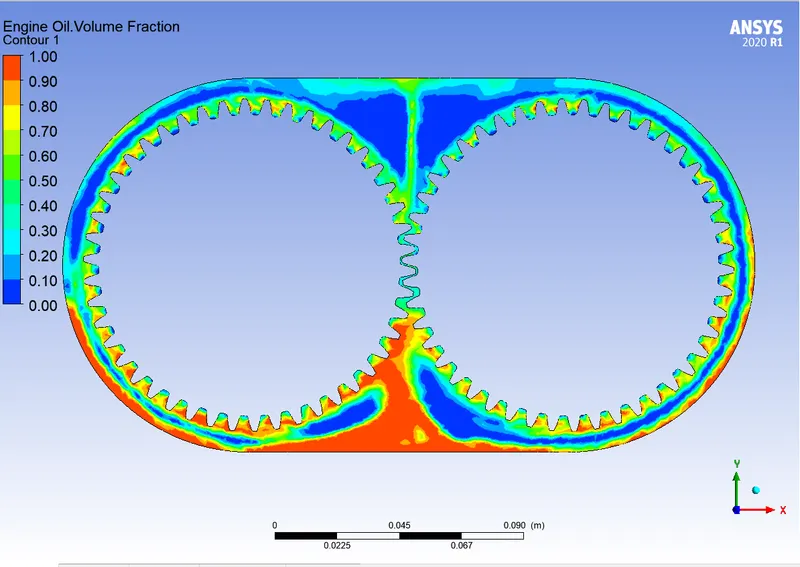
30% Immersion, Fluid- Engine oil:

20% Immersion,Fluid-n-heptane:

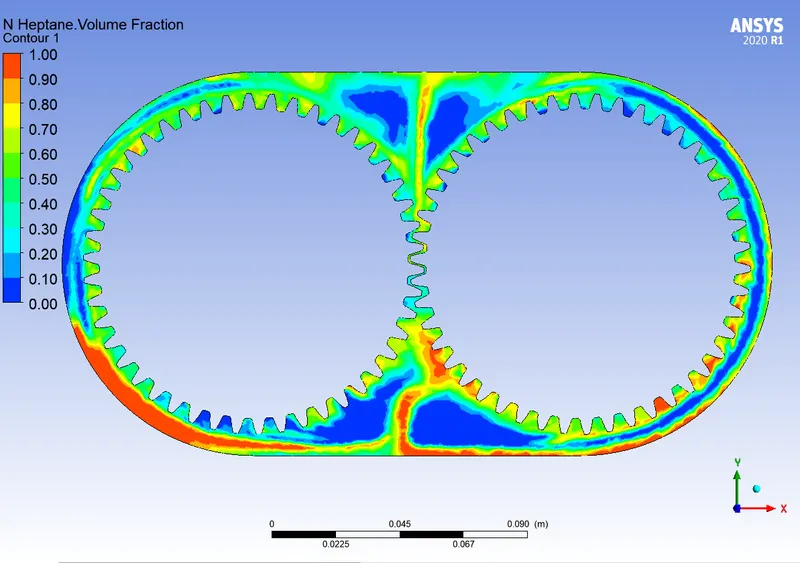
30% Immersion,Fluid-n-heptane:

Tabulated comparison of 1500th timestep of each case:

	20% Immersed	30% Immersed
Engine Oil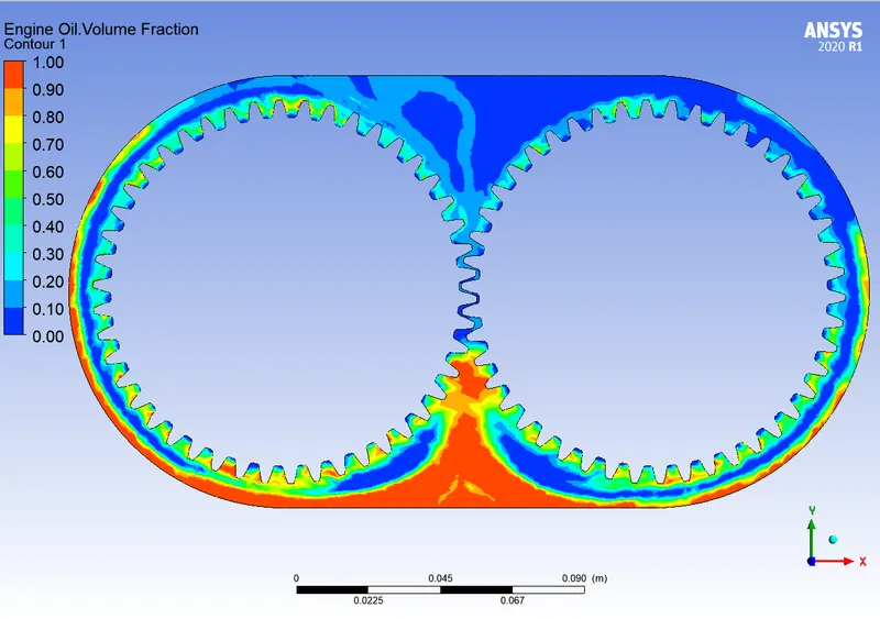
n-Heptane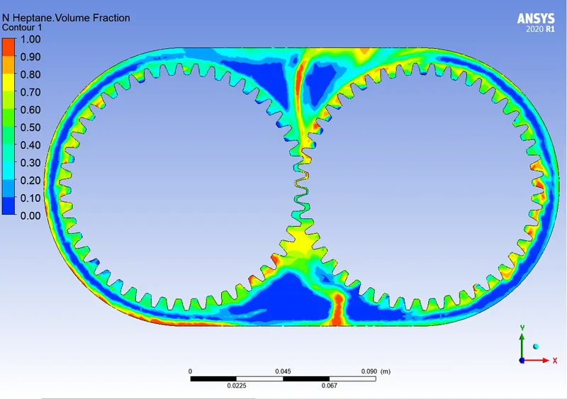

CONCLUSION:

The volume fraction of the respective fluids was plotted as a function of time, and the lubrication of the gear teeth was observed.

Better sloshing resulted in better lubrication of n-Heptane on the gear teeth.

30% Immersed fluid showed better lubrication than its conuter 20% Immersed fluid.

Sloshing effect is lesser in Engine Oil is less compared to n-Heptane because of viscosity variation.

The results are applicable upto certain case considerations, and required more refinement and features to get the bigger practical picture.