CFD Simulation of Combustor Model to analyze Emissions and Soot Formation
CFD SIMULATION OF COMBUSTOR MODEL TO ANALYZE EMISSIONS AND SOOT FORMATION
AIM:
- Perform a combustion simulation on the combustor model and plot the variation of the mass fraction of the different species’ in the simulation using line probes at different locations of the combustor as shown in Fig. You need to plot for CO2, H2O, CH4, N2, O2, NOx emissions & Soot formation.
- As you must have observed from the above simulation, the Nox and soot is getting formed at the outlet of the combustor. Such formation has harmful effects on the environment and humans. The stringent government norms also demand the least formation of Nox and soot and to satisfy those requirements, you need to check the effect of adding the water in the fuel. In this part, you need to add the water content in the fuel from 5% to 30% by mole and observe the effect of it on the results. It is necessary to provide line plots and contours to prove your claim. You can use the parametric study approach if required.
INTRODUCTION:
A combustor is a component or area of a gas turbine, ramjet/scramjet engine where combustion takes place. It is also known as a burner, combustion chamber or flame holder. In a gas turbine engine, the combustor or combustion chamber is fed high pressure air by the compression system. The combustor then heats this air at constant pressure. After heating, air passes from the combustor through the nozzle guide vanes to the turbine. In the case of a ramjet or scramjet engines, the air is directly fed to the nozzle.
A combustor must contain and maintain stable combustion despite very high air flow rates. To do so combustors are carefully designed to first mix and ignite the air and fuel, and then mix in more air to complete the combustion process. Early gas turbine engines used a single chamber known as a can type combustor. Today three main configurations exist: can, annular and cannular (also referred to as can-annular tubo-annular). Afterburners are often considered another type of combustor.
Combustors play a crucial role in determining many of an engine's operating characteristics, such as fuel efficiency, levels of emissions and transient response (the response to changing conditions such as fuel flow and air speed).
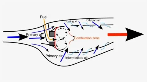
Fig.1 Schematic of a combustor
Various types of Combustion simulations are available Based on Mixing, Based on Phase and Based on Equation Solved. The Species Transport equation is used for the current simulation:
`del/(delt)(rhoY_i)+grad.(rhovecvY_i)=-grad.vecJ_i+R_i+S_i`
where `Y_i`represents the Mass fraction of the species.
In comparison between the Laminar and Turbulent Diffusion models, the later is a dominant factor. Therefore, Dilute approximation can be considered for the current case, wherein the Laminar Diffusion is neglected and only Turbulent is siumlated. The Combustion Source Calculation involves Eddy Disipation Model, as it is a mixing based model. It initiates the combustion based on the turbulence observed in the combustor.
The equation used for the chemical kinetics is:
`CH_4+2(O_2+3.76N_2)rarrCO_2+2H_2O+7.52N_2`
The Mole fraction of `O_2` is t be input into the air-Inlet boundary condityion. Based on the stoichiometric reaction, the mole and mass fraction vales are extracted.
`text(Mole Fraction of ) O_2=(text(Moles of )O_2)/(text(Moles of Air)(N_2+O_2))=2/(2+7.52)=0.21`
The background for this simulation is the increasingly stricter limits set for the emission of the toxic exhaust gas components by marine engines. Legal requirements force designers to search for new constructions of marine propulsion systems and constantly improve the existing ones. One of the solutions is supplying water into the combustion chambers of diesel engines—the solution widely known for many years now wins favour and, according to the authors, has a chance to gain competitive advantage over alternative constructions.
SOLVING AND MODELLING APPROACH:
The following flow chart is followed for the Solving Approach:
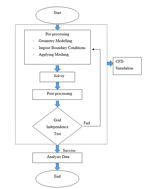
Fig.2 Solving Approach Flow Chart
ANSYS involves selection of Fluent solver, input and verification of Geometry, Meshing, Setup, Solutions and Results. The Geometry is input in ANSYS Space Claim. The mesh sizing and face naming is done while Meshing. The Setup section involves Mesh Checking, Turbulence Model selection, Solver type, velocity formulation and time (steady or transient state), Output report files, Material selection, Initial and Boundary conditions. The Results section is used for the visualiztion of the output in a GUI.
PRE-PROCESSING AND SOLVER SETTINGS:
GEOMETRY:
(a) (b)
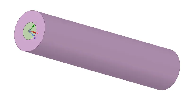
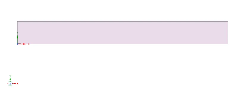
Fig.3 (a)CAD Geometry for Combustor ,(b) 2D geometry of Combustor
The above geometry is imported into Spaceclaim. The Split Body command is used to split the geometry along XZ and XY plane. The quadrant face obtained is copied into a new geometry. The Combine option was used to join all the individual faces.
MESHING:
(a) (b)
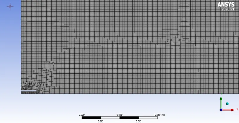
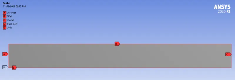
Fig.4 (a)Meshing for the Geometry
A baseline mesh was created with element size of 2mm. The respective faces were named Inlet, Outlet, Axis and Wall. The Capture Proximity module in Sizing is switched on and the number of cells is set to 5.
SETUP:
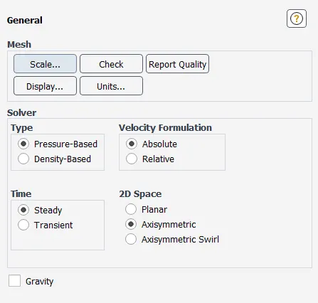
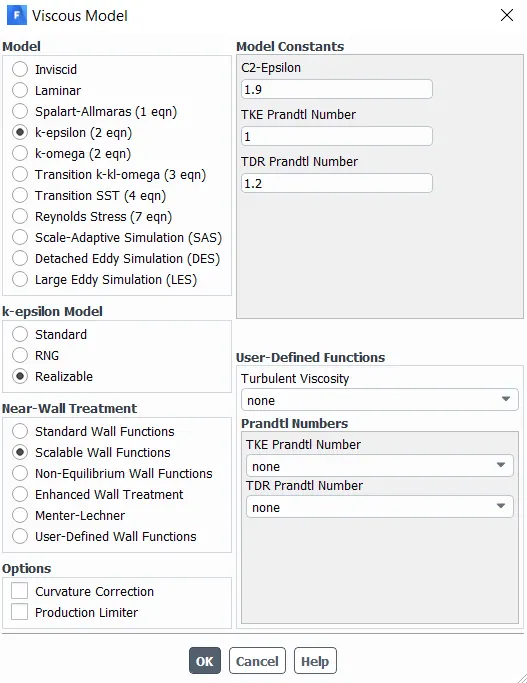
Since the problelm statement is considered for a low Mach number, a Pressure Based Solver is considered for the simulation. The `k-epsilon` Standard Turbulence model was used for the respective test case calculations. The Axisymmetric Module is enabled.
(a) (b)
Fig.5 (a)Setup- General, (b) Setup- Viscous Model
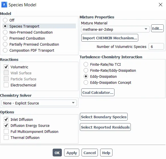
A Steady State simulation is run. The Energy option is enabled for temperature derivations. In the Physics section, Species tab is selected and Species Transport is enabled. The Volumetric Reactions are turned on, and Inlet Diffusion is opted. Eddy Dissipation is switched on in Turbulence-Chemistry and Methane-Air 2 Step (Allows water mass fraction input in boundary conditions) mixture is selected as mixture material.
(a) (b)
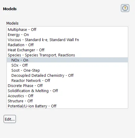
Fig.6 (a)Setup-Species Modeling (b) Setup- Models to be considered for the simulation
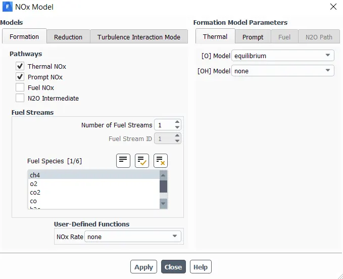
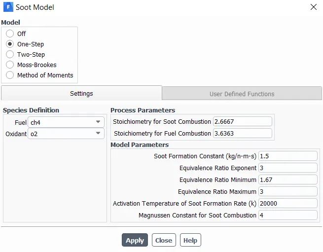
The NOx and Soot Modeling were setup. Thermal and Prompt pathways were enabled in NOx. The fuel species was selected as `CH_4`. The Soot Model was set to One-Step Model and the Fuel was set to `CH_4` and Oxidant to `O_2`. The remaining parameters were left to default.
(a) (b)
Fig.7 (a) Setup Models- NOx (b) Setup Models- Soot
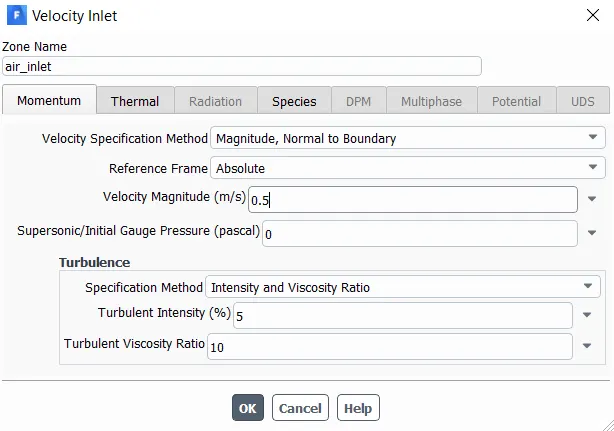
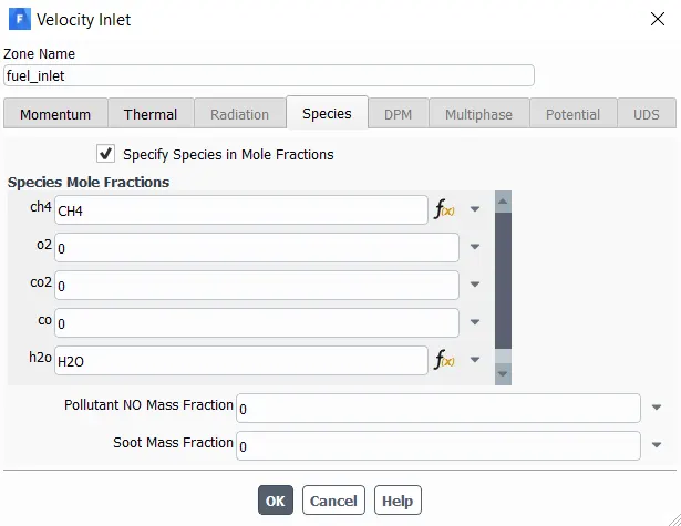
For Boundary Conditions, the Air-Inlet is given a velocity-inlet input with 0.5 m/s. The temperature set to 300 K. The species is given a mass fraction value of 0.23 for `O_2`. The Fuel-Inlet is given a velocity-inlet input with 80 m/s. The temperature set to 300 K. The species is given a mass fraction value of 1 for `CH_4` and 0 for `H_2O` A New Paramter was created for the methane and water mass fractions. These values will be input in the parametric study of other cases. The Outlet is automatically given a gauge pressure of 0Pa. The mass fractions were derived from the stoichiometric equation of the combustion reaction.
(a) (b)
Fig.8 Boundary Condition Setup- (a) Air Inlet Velocity Input (b) Fuel Species Mass Fraction Input
The Hybrid Initialization is used to intialize. In Definitions, New Surface Report is created for Total Temperature, Mass Fraction of Soot and NOx at the Outlet using Area-Weighted Average computation. The Create Output Parameter is used on all the three output parameters to set this as the output varying, dependent on the input parameters.The simulation is run for 500 iterations.
RESULTS:
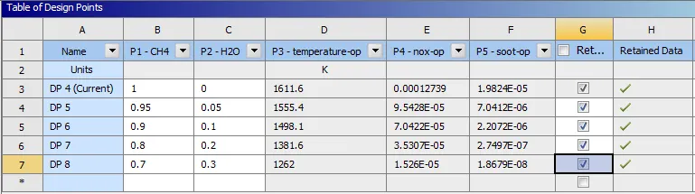
Table 1: Parametric Study for the input `CH_4 and H_2O` mole fractions and output `NO_x` and Soot
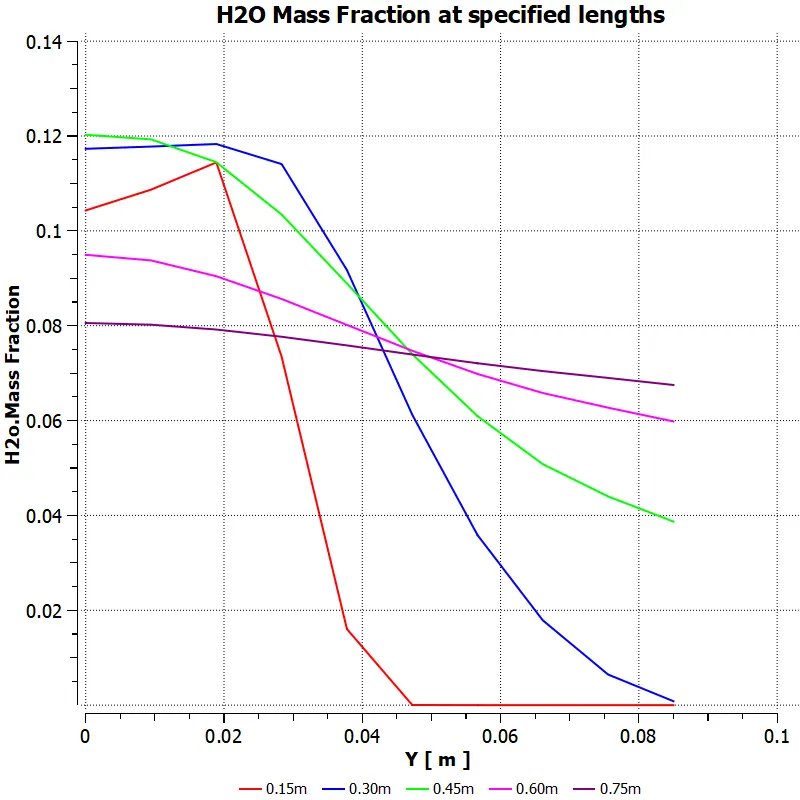
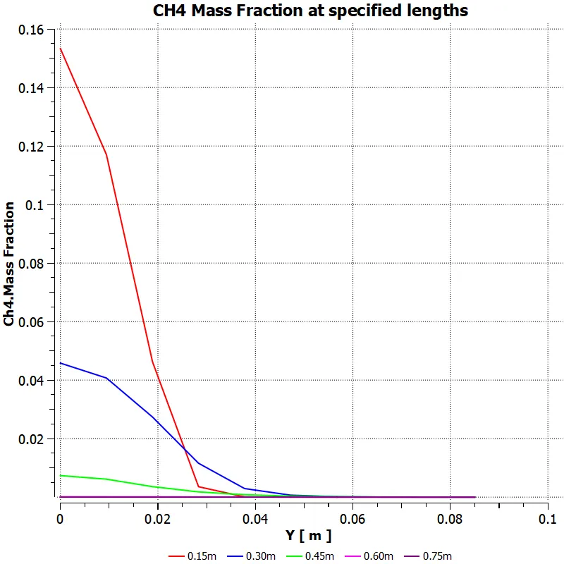
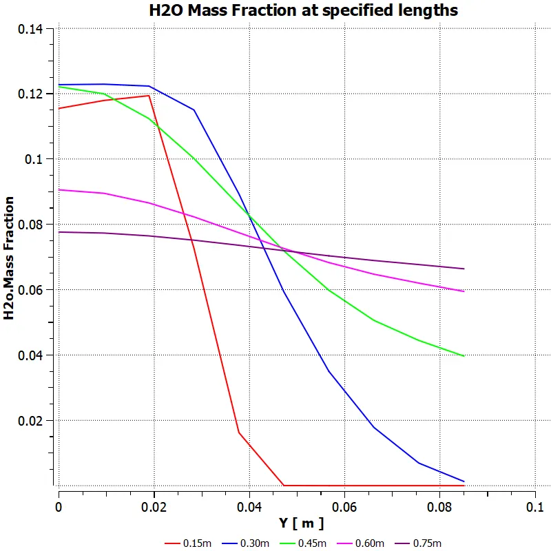
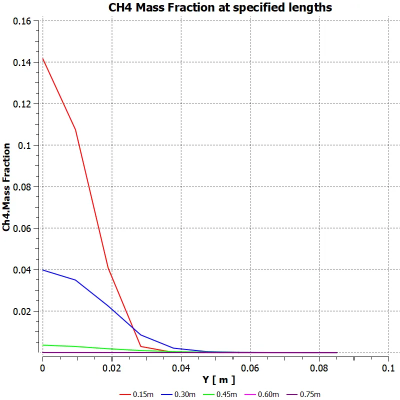
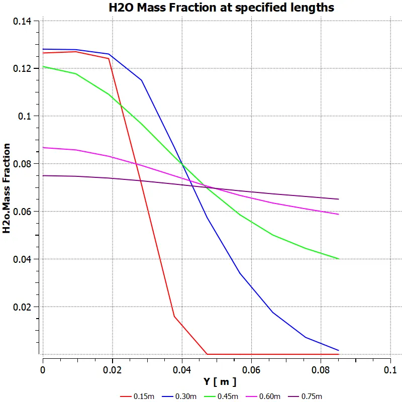
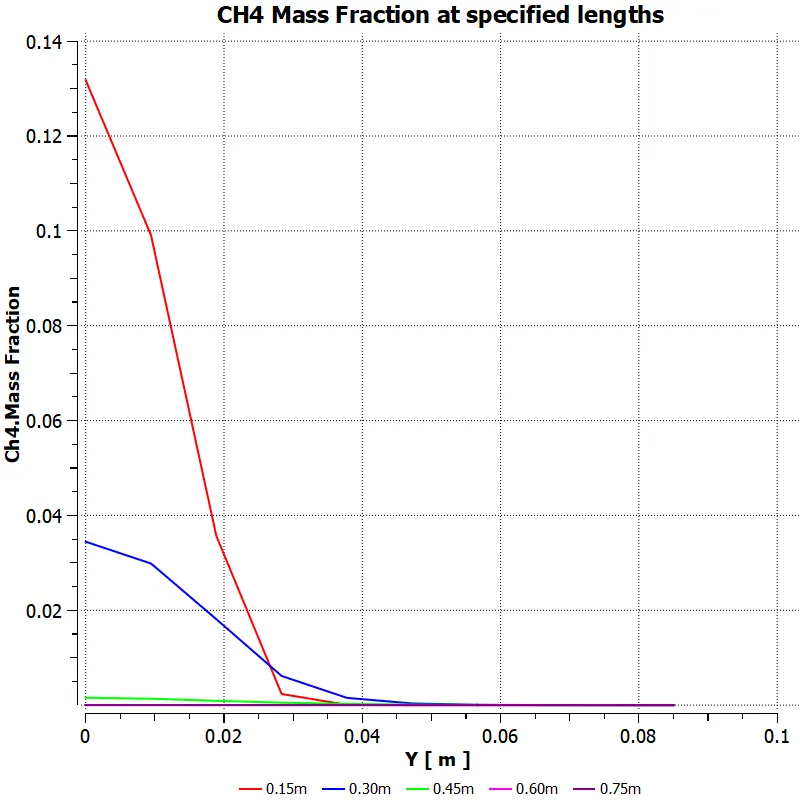
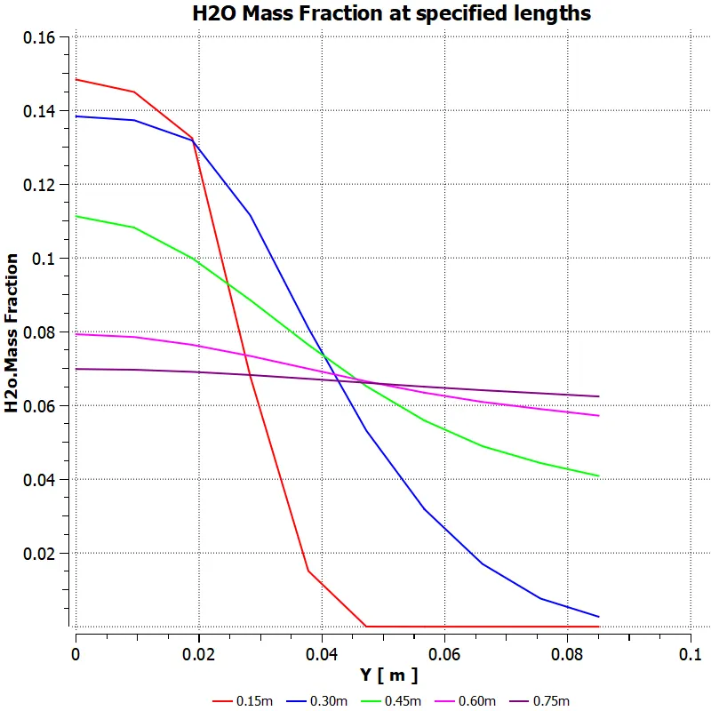
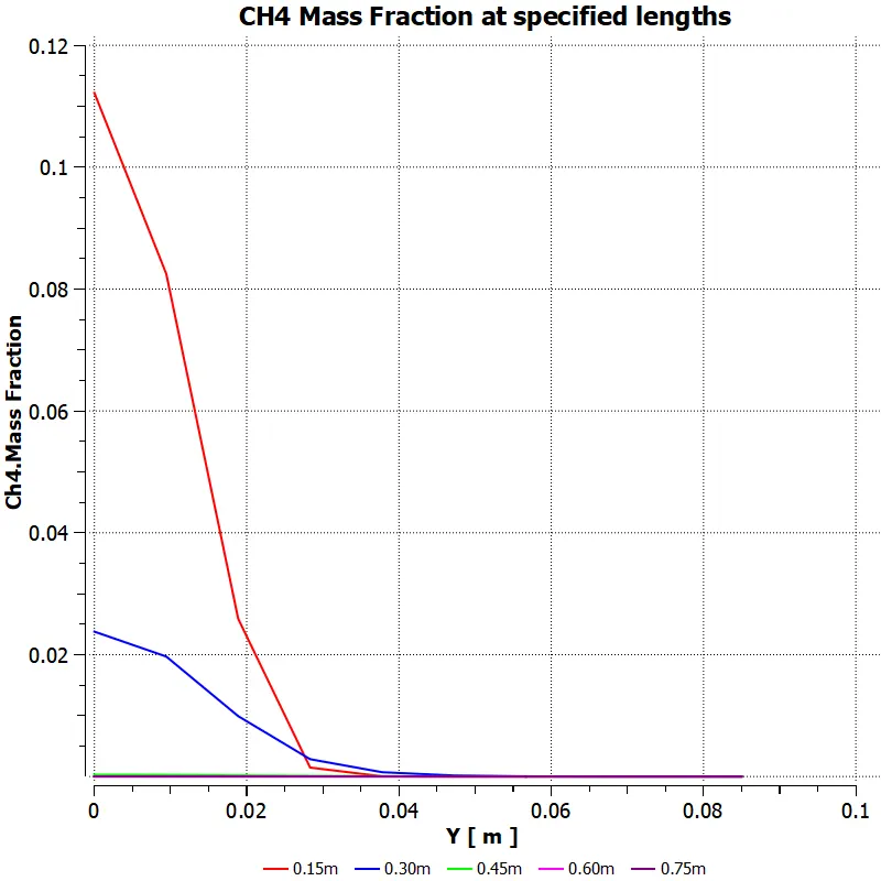
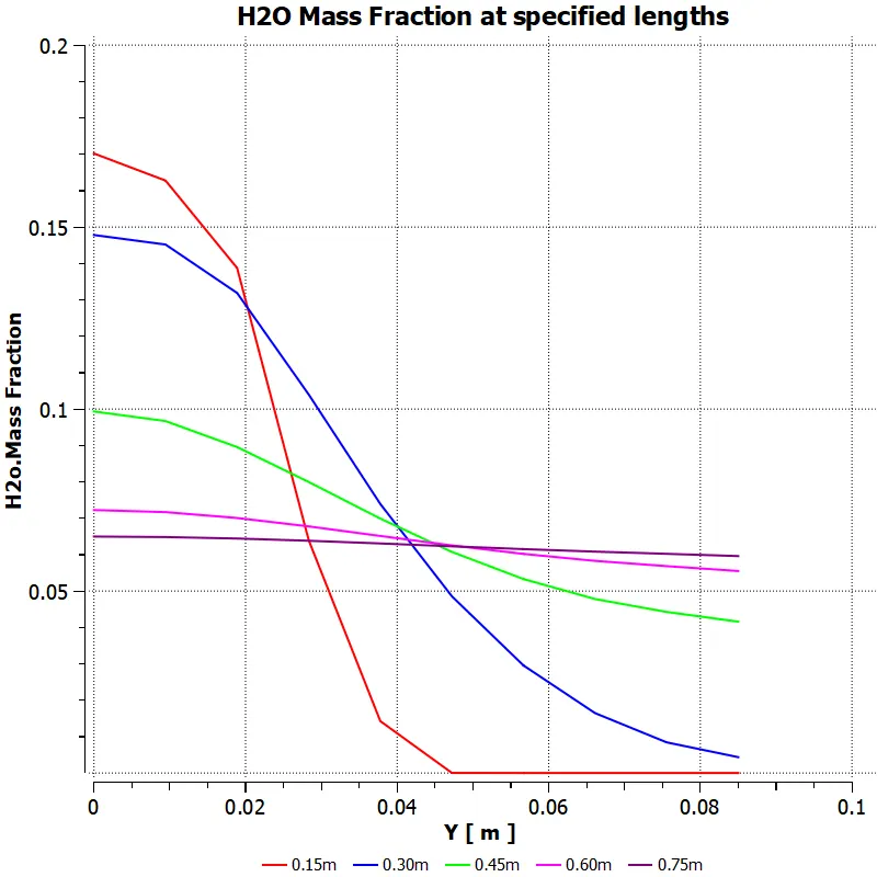
The following lines were created along the cross-section of the combustor to obtain the respective residual mass fractions:
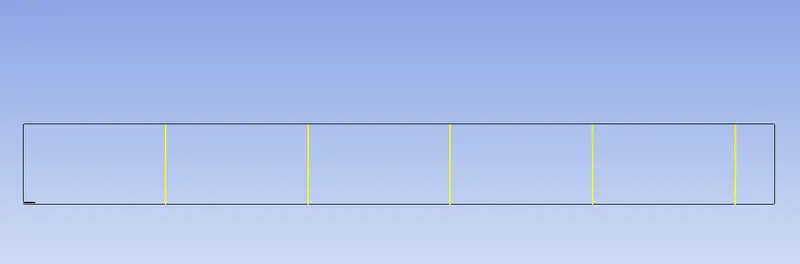
Fig.9 Lines placed at 0.15m, 0.30m, 0.45m, 0.60m and 0.75m
Table 2: Temperature contours observed for test cases
| Test Case | Temperature Contours |
| Water Mole Fraction 0% | 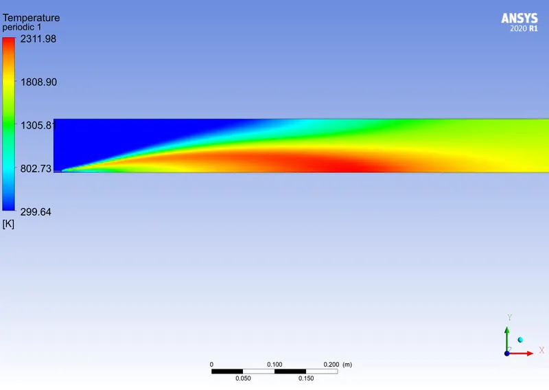 |
| Water Mole Fraction 5% | 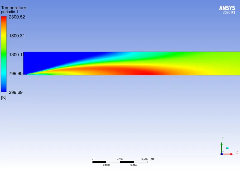 |
| Water Mole Fraction 10% | 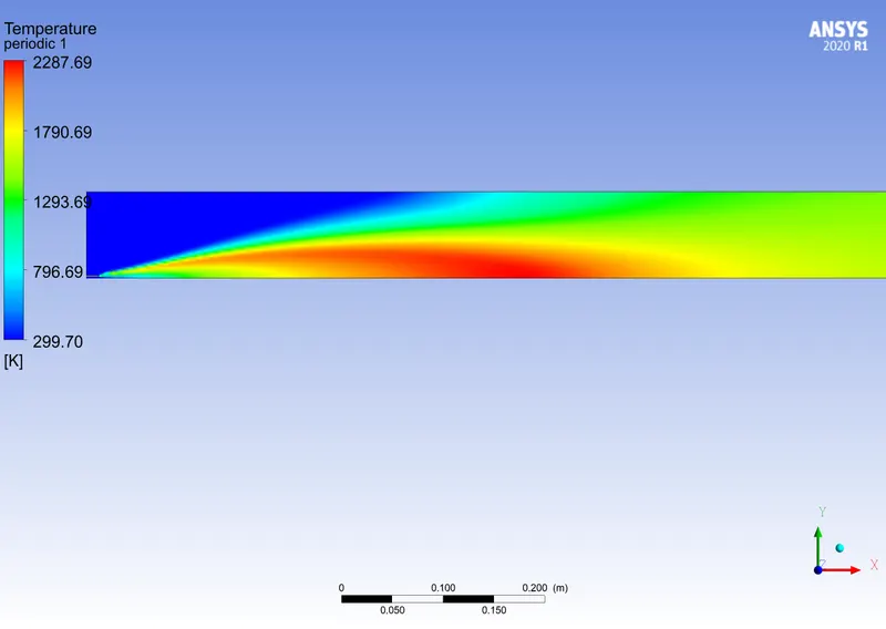 |
| Water Mole Fraction 20% | 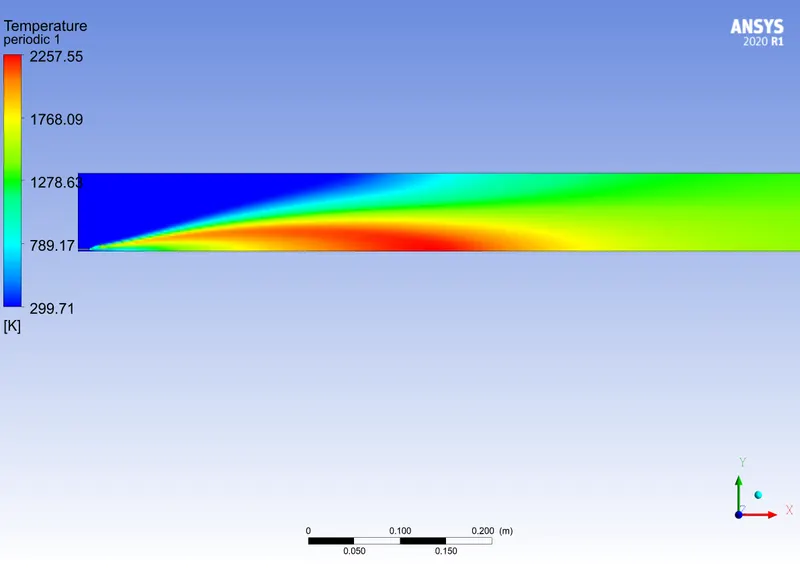 |
| Water Mole Fraction 30% | 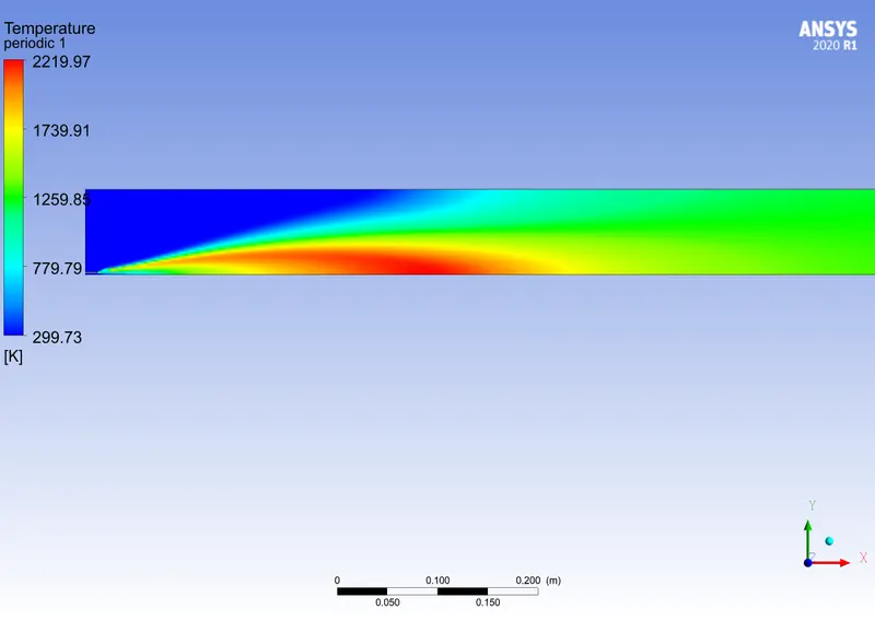 |
Table 3: `CO_2`,`H_2O` and `CH_4` Mass Fraction plots at specified lines in combustor
| Water Mole Fraction 0% | 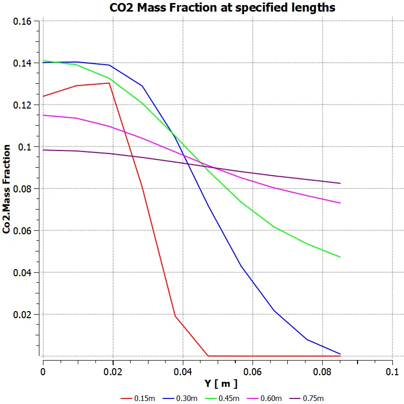 |
 |
 |
| Water Mole Fraction 5% | 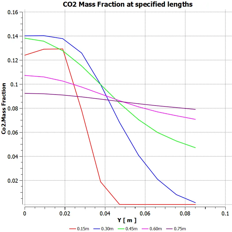 |
 |
 |
| Water Mole Fraction 10% | 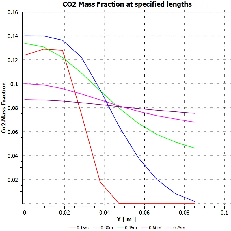 |
 |
 |
| Water Mole Fraction 20% | 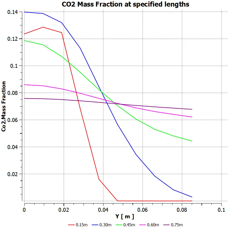 |
 |
 |
| Water Mole Fraction 30% | 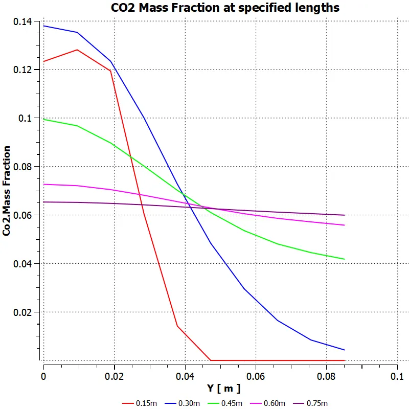 |
 |
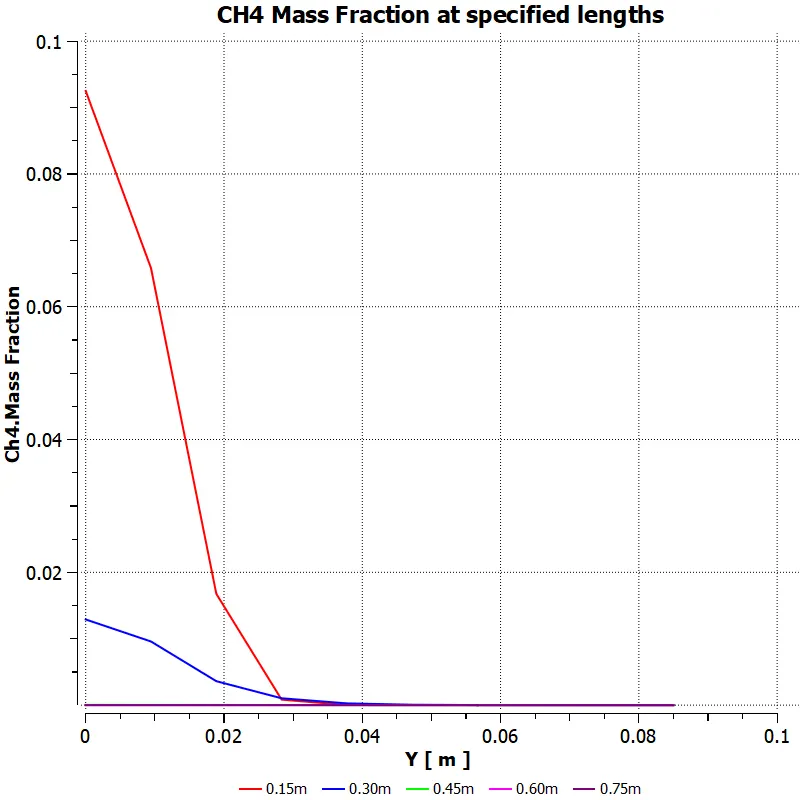 |
Table 4: `N_2,O_2` Mass Fraction plots at specified lines in combustor
| Water Mole Fraction 0% | 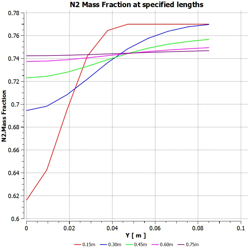 |
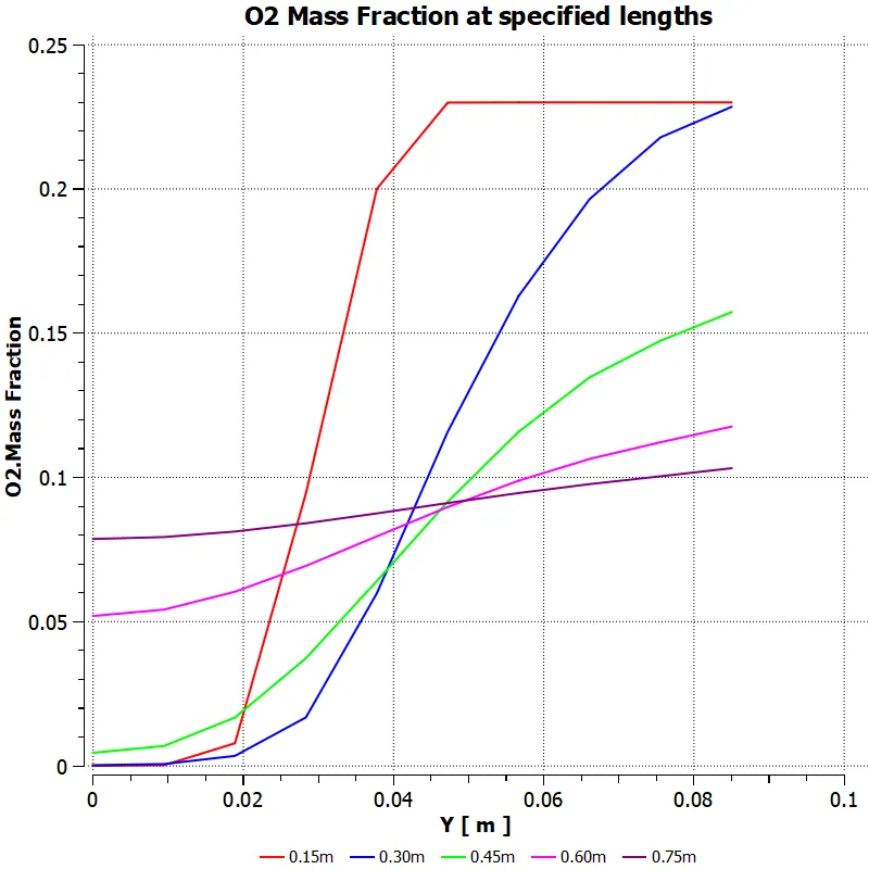 |
| Water Mole Fraction 5% | 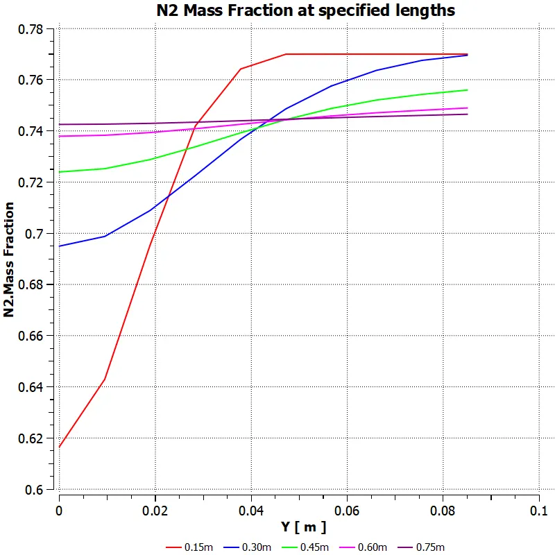 |
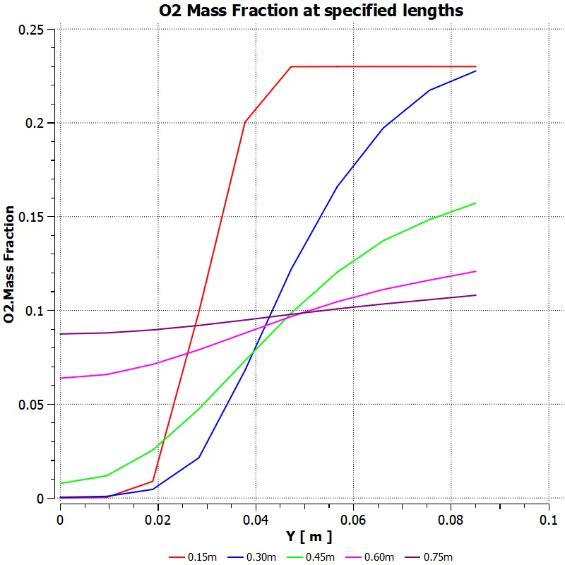 |
| Water Mole Fraction 10% | 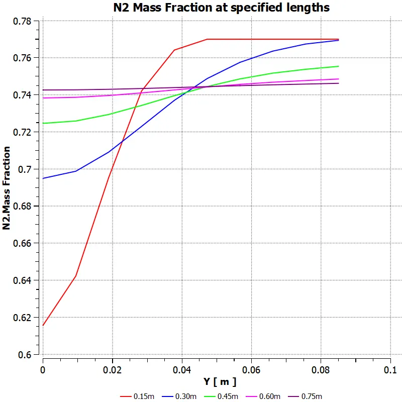 |
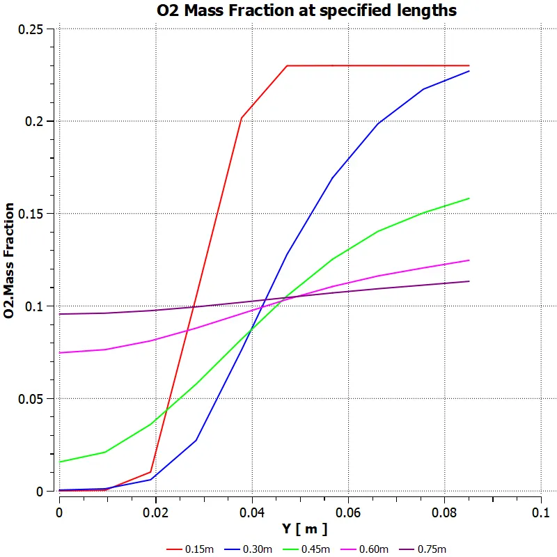 |
| Water Mole Fraction 20% | 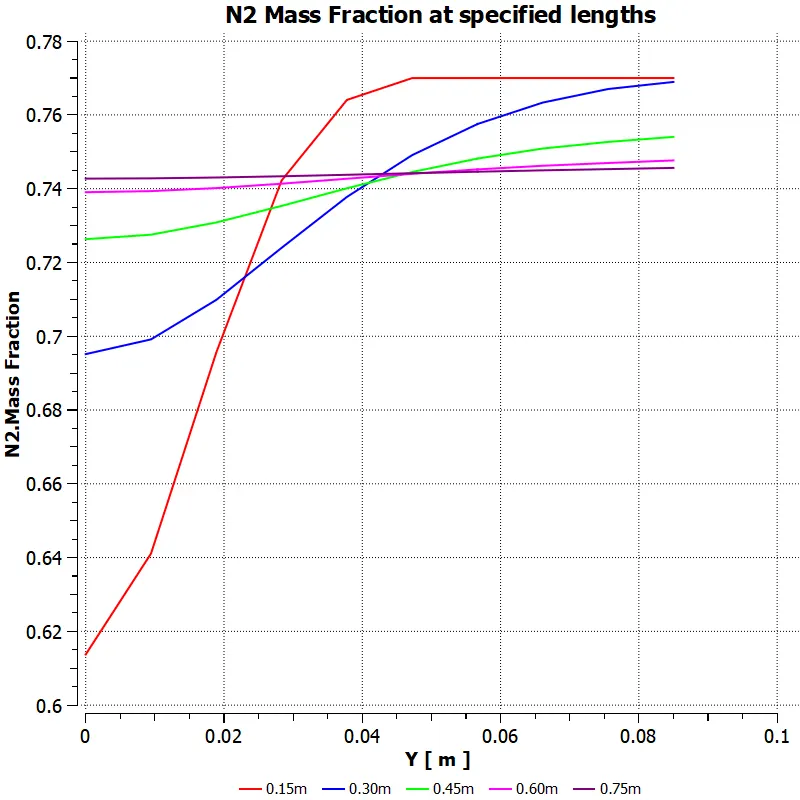 |
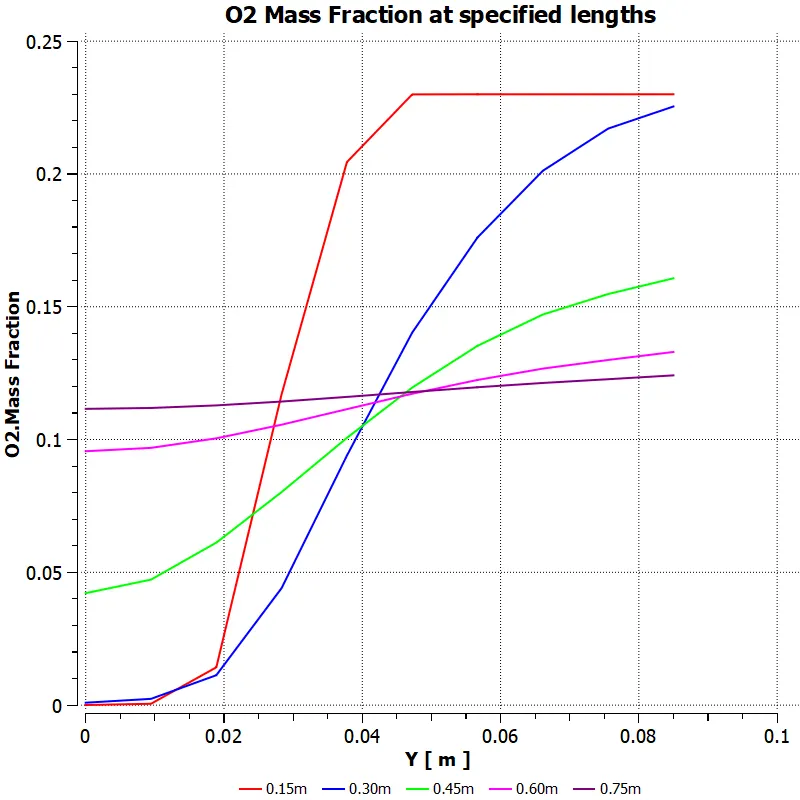 |
| Water Mole Fraction 30% | 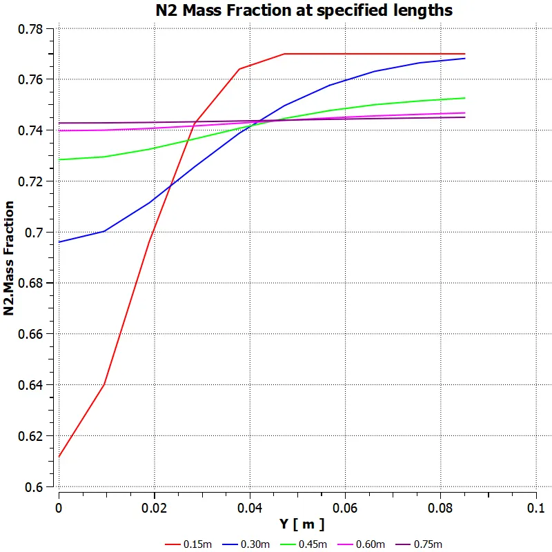 |
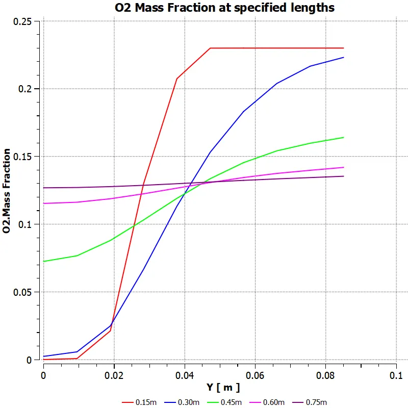 |
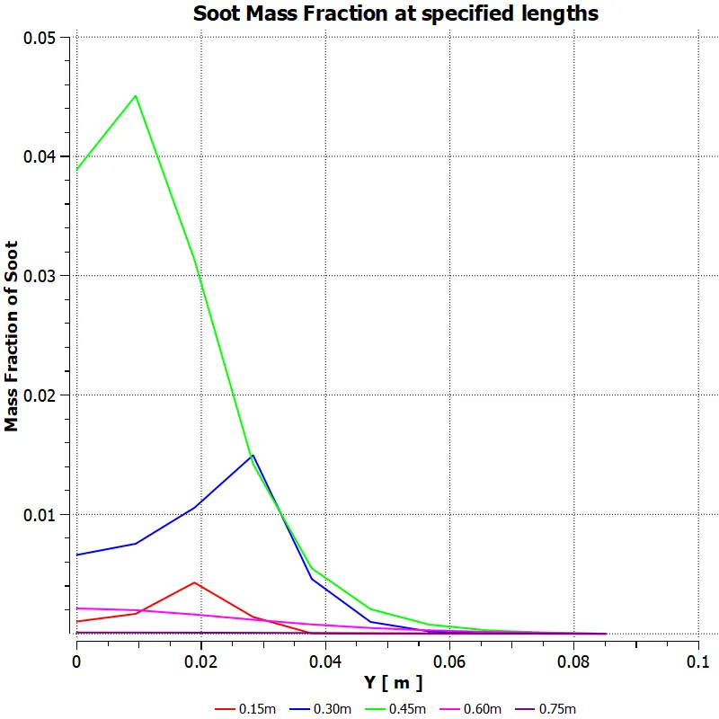
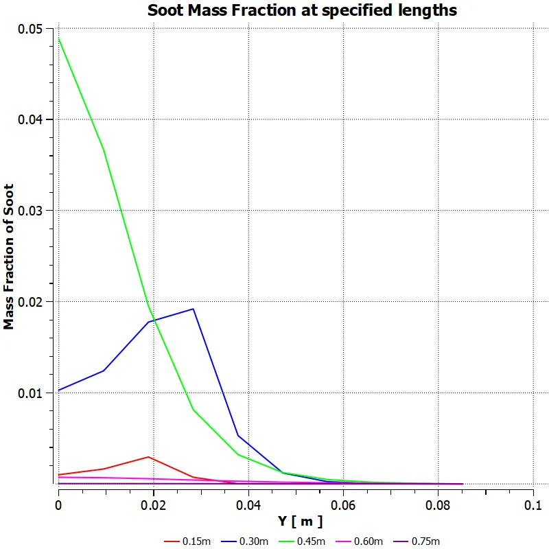
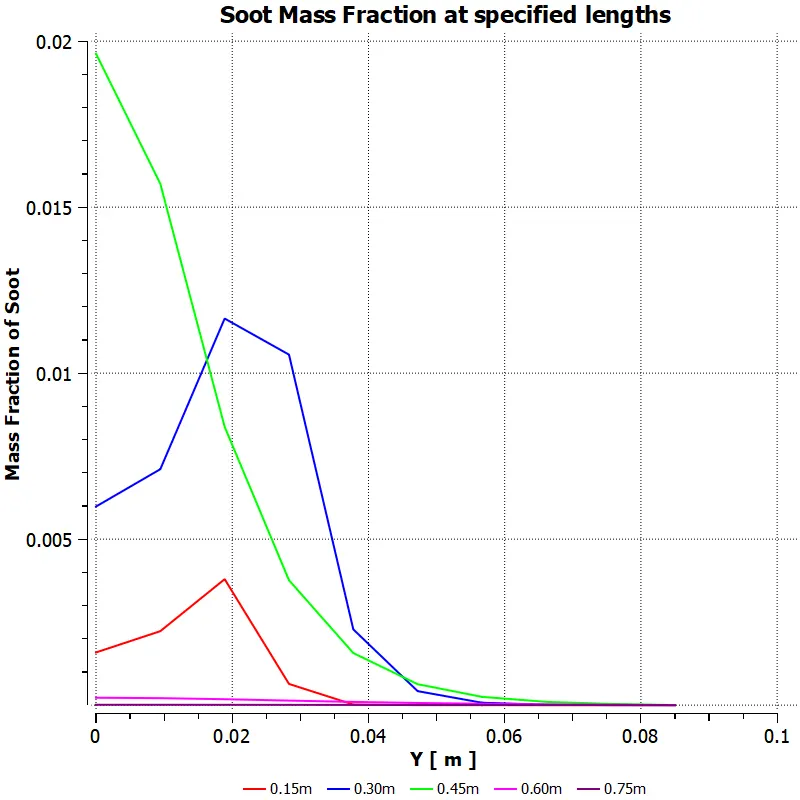
Table 5: `NO_x,text(Soot)`Mass Fraction plots at specified lines in combustor
| Water Mole Fraction 0% | 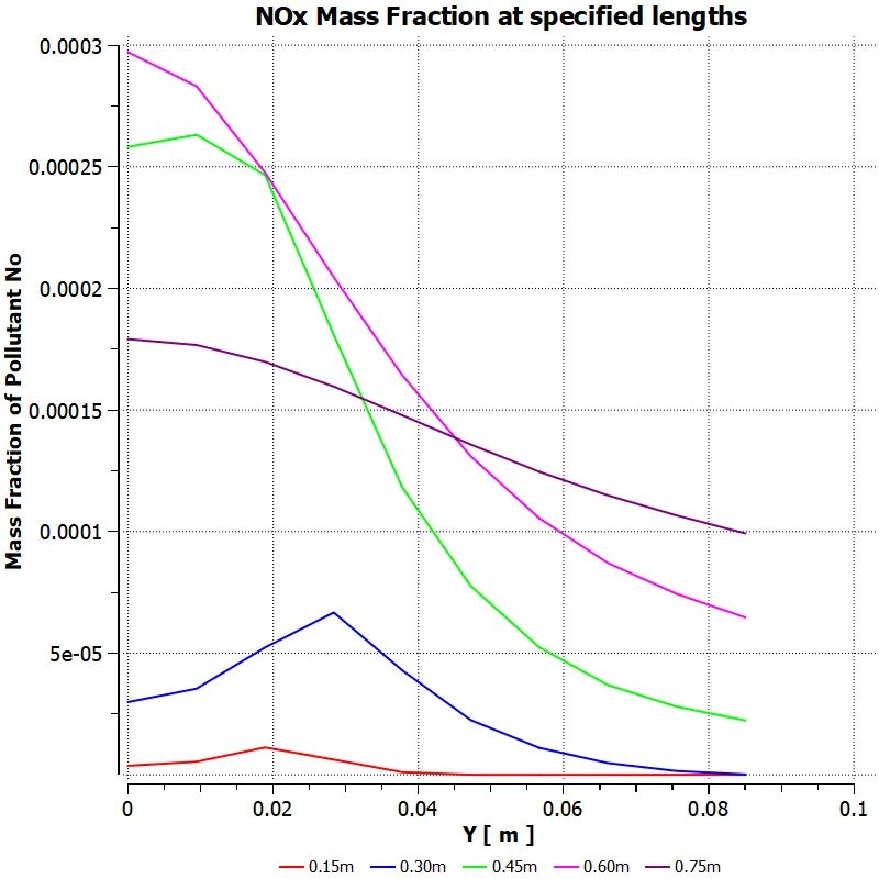 |
 |
| Water Mole Fraction 5% | 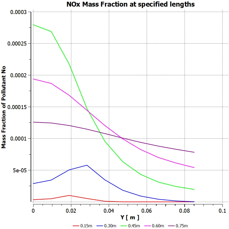 |
 |
| Water Mole Fraction 10% | 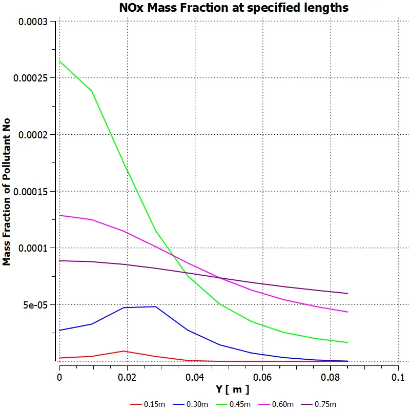 |
 |
| Water Mole Fraction 20% | 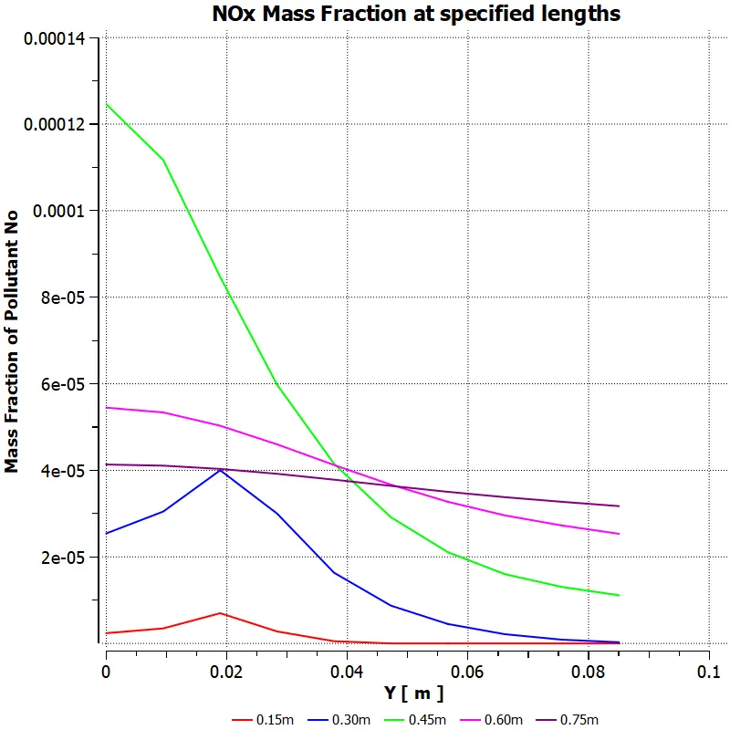 |
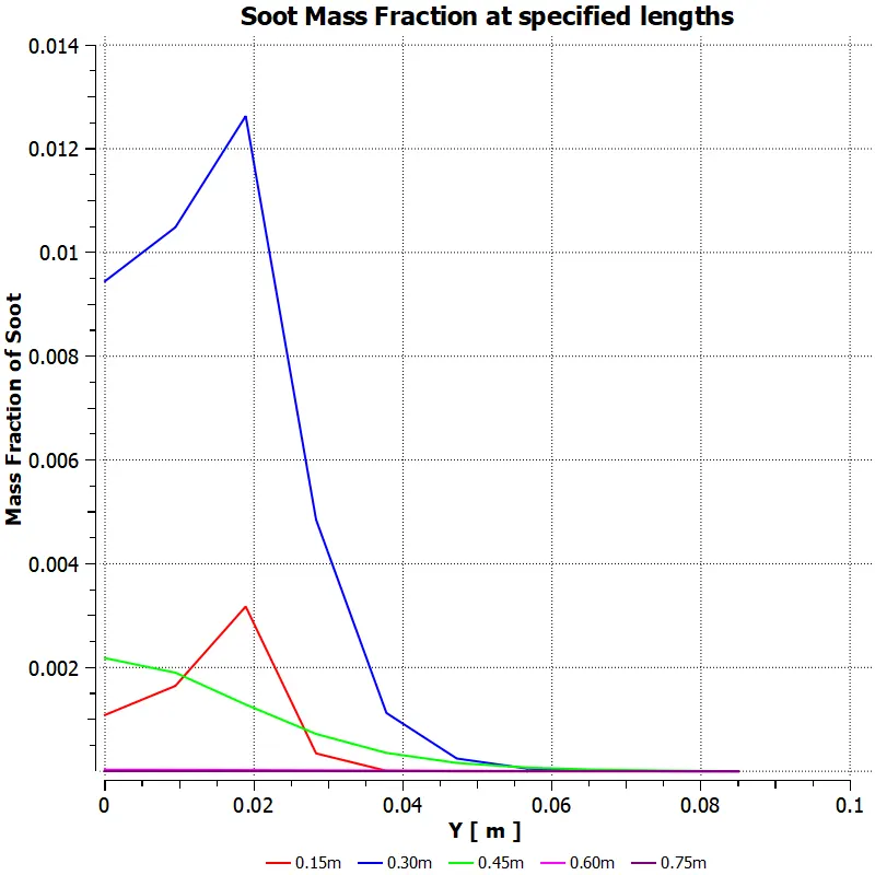 |
| Water Mole Fraction 30% | 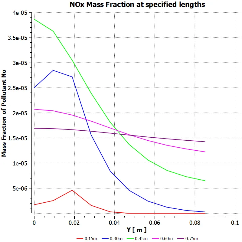 |
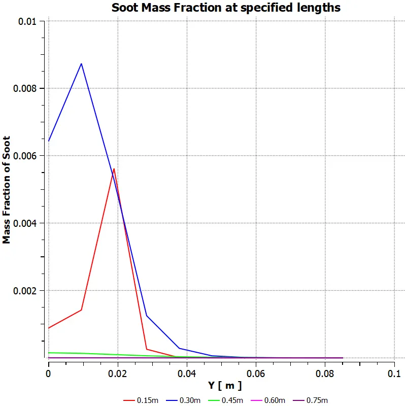 |
CONCLUSION:
It is observed that the outlet total temperature is decreasing as the mole fraction of water at the inlet increases.
The `NO_x` and Soot Mass Fractions also reduced as the water mole fraction was increased.
The maximum temperature reached by the combustor is also reduced by the increase in water input mole fraction.
The `NO_x` and Soot mass fractions reduce gradually as thealong the axis and the radial lines.