ITERATIVE SOLUTION USING LINEAR ALGEBRA IN MATLAB

UNDERSTANDING LINEAR SYSTEMS

AIM:

• Solve the system of matrices using Jacobi, Gauss-seidel and SOR methods.
• Compute the Iteration Matrix for the above mentioned methods by suitable matrix decomposition techniques taught in the lectures.
• Calculate the Eigen values of the Iteration matrix.
• Calculate the Spectral radius of the Iteration matrix.
• Introduce a suitable scaling factor called diagonal magnification factor that scales the given diagonal elements within a range, say [0.1:0.1:2] for answering question

OBJECTIVES OF THE PROJECT:

• The Eigen values and Spectral radius is discussed in theory. The iteration formula for each method is extracted from literature.
• The Iteration matrix is extraccted for each iteration method and the spectral radius for each is calculated for comparison.
• A scaling factor is interoduced to observe the variation of spectral radius and number of iterations for each method as a function of diagonal elements.

ANSWERS TO QUESTIONS:

1) Explain the concept of Eigen value & Spectral radius of the matrix. How does it affect the convergence rate of the solution?

1. A) For any matrix `A'`, a set of eigen values are present denoted by vector `lamda`, which can be expressed as:

`(A'-lamdaI)X=0`

where `X` is the Eigen vector for the matrix. An eigenvector, corresponding to a real nonzero eigenvalue, points in a direction in which it is stretched by the transformation and the eigenvalue is the factor by which it is stretched(by the eigenvalue). Solving for `lamda` from `|A-lamdaI=0|`,

`lamda^3-Alamda^2+Blamda-C=0`

where: `A` is the trace of the original matrix , `B` is the sum of minors of diagonal elements, and `C` is the determinent of matrix `A'`.

Spectral Radius refers to the maximum absolute value amongst the computed eigenvalues, and is denoted as `rho`. Lower the spectral radius (`rho<1`), better is the convergence for the iteration, and lower number of iterations are required for the convergence. The value of the spectral radius is effected by the diagonal elements of the iteration matrix, which will be varied by a factor to observed the relationship of the factor with the convergence of the solution.

2) What is Diagonal dominance? How do the diagonal terms of an Iteration matrix affect the solution through iterative methods? Is there a relationship between Diagonal dominance and spectral radius ?

1. A) Diagonal dominance refers to the magnification of the diagonal terms in the iteration matrix. As discussed, this is done by a scaling factor, multiplied to the matrix. Theroitically, the higher the values of diagonal elements or higher the magnification factor, lower is the spectral radius and better is the convergence of the iterative solution. Better convergence refers to lower number of iterations to reach the best solution. The diagonal elements are introduced in the matrix `D`, which is used for the iterative computation. The next section describes the formulaes for the iteration formulaes, wherein it can be seen that the matrix `D` plays a crucial role in every iterative step. hence, increasing the values in the diagonal elements, increases the rate at which the `x_(text(new))` is updated from the `x_(text(old))` values.

GOVERNING EQUATIONS:

Iterative methods involve, guessing of initial values of the required variable set, and computing the new values on a loop. When the error of the latest values reaches an appreciable value, the solution is obtained.

Solving for the equation `AX=B`, where `A=U+L+D`, and `U` represents the upper triangular matrix of `A`, `L` represents the lower triangular matrix of `A` and `D` represents the diagonal elements matrix of `A`.

The iteration formulae for each method is:

Jacobi: `x^(k+1)=D^(-1)(B-(U+L)x^((k)))`

Gauss Seidel: `x^(k+1)=(L+D)^(-1)(B-Ux^((k)))`

SOR: `x^(k+1)=(D+omegaL)^(-1)[omegaB-(omegaU+(i-omega)D)x^((k))]`

where `x^((k))` represents the `k^(th)` iteration step and `x^((k+1))` represents the `(k+1)^(th)` iteration step.

The `omega` in the Relaxation method is used for the faster convergence of the iteration on whichever method it is used upon. In this case the Gauss Seidel method is used in SOR:

`omega=2-2/(sqrt(1-mu^2))`

where `mu` would represent the spectrl radius obtained from the Gauss Seidel iteration matrix.

The iteration matrix for the computation of each spectral radius of each matrix is as follows:

Jacobi: `D^(-1)(L+U)`

Gauss Seidel: `(L+D)^(-1)U`

SOR: `(D+omegaL)^(-1)[omegaU+(1-omega)D]`

It should be noted that the spectral radius of the respective matrix will converge faster for lower values (`rho<1`) .

BODY OF THE CONTENT:

CODE:

clear all,close all, clc
%Convergence study on iterative methods
%The original transformation matrix is fragmented into U,L and D.
U=[0,1,2;0,0,4;0,0,0];
L=[0,0,0;-3,0,0;1,2,0];
D=[5,0,0;0,9,0;0,0,-7];
A=U+L+D;
%The solution matrix B is input
B=[10;-14;33];
%Eigen Value of Matrix
%To solve for the eigenvalues, the parameters as listed in the cubic
%equation should be solved.
%trace() gives the trace of the matrix
a=trace(A);
b=0;
%Below is the loop considering the minors of each diagonal elements and 
%adding into b. 
for i=1:length(A)
   M=A;
   M(i,:)=[];
   M(:,i)=[];
   K=det(M);
   b=b+K;
end    
%det() is used to calculate the determinent of matrix.
c=det(A);
%The coefficients are put in a vector coeff.
coeff=[1 -a b -c];
%roots() command gives the roots considering the coefficients input to 
%solve the equation. 
%The computed roots are stored in eigen_values. Taking the absolute maximum
%of this vector gives the spectral radius.
eigen_values=roots(coeff);
%Diagonal Increament factor
I=0.4:0.2:1.2;
%D_old is described as an initial matrix for multiplying the magnification
%factor
D_old=D;
%A loop is run for each magnification factor
for i=1:length(I)
    %The factor is multiplied to the diagonal elements
    D=I(i)*D_old;
    %The iteration matrix is computed from the respective formulas
    Iteration_jac=inv(D)*(L+U);
    %The eigenvalues are computed using the inbuilt eig function. And the
    %spectral radius is found by computing the absolute maximum of the eigen
    %values.
    rho_jac(i)=max(abs(eig(Iteration_jac)));
    
    Iteration_gs=inv(D+L)*(U);
    rho_gs(i)=max(abs(eig(Iteration_gs)));
    %For SOR, the omega is computed 
    w=2-(2/(1+sqrt(1-rho_gs(i)^2)));
    Iteration_sor=inv(D)*(L+U);
    rho_sor(i)=max(abs(eig(Iteration_sor)));
    %An initial guess vector for coefficients is input
    x_old=[0;0;0];
    %The matrices along with x_old is input for computation.
    [iternum_jac(i),x_jac]=jacobi_iteration(A,B,U,L,D,x_old);
    [iternum_gs(i),x_gs]=gs_iteration(A,B,U,L,D,x_old);
    [iternum_sor(i),x_sor]=sor_iteration(A,B,U,L,D,x_old,w);
    
end    

%Plotting
%Plot for Jacobi Iteration
figure(1)
subplot(3,1,1)
plot(I,rho_jac)
xlabel('Spectral Magnification')
ylabel('Spectral Radius')
axis([0.4 1.2 0 3])
grid on
title('Jacobi Iteration')
subplot(3,1,2)
plot(rho_jac,iternum_jac)
xlabel('Spectral Radius')
ylabel('Number of Iterations')
axis([0 3 0 3000])
grid on
subplot(3,1,3)
plot(I,iternum_jac)
xlabel('Spectral Magnification')
ylabel('Number of Iterations')
axis([0.4 1.2 0 3000])
grid on

%Plot for Gauss Seidel Iteration
figure(2)
subplot(3,1,1)
plot(I,rho_gs)
xlabel('Spectral Magnification')
ylabel('Spectral Radius')
axis([0.4 1.2 0 3])
grid on
title('Gauss Seidel Iteration')
subplot(3,1,2)
plot(rho_gs,iternum_gs)
xlabel('Spectral Radius')
ylabel('Number of Iterations')
axis([0 3 0 3000])
grid on
subplot(3,1,3)
plot(I,iternum_gs)
xlabel('Spectral Magnification')
ylabel('Number of Iterations')
axis([0.4 1.2 0 3000])
grid on

%Plot for SOR Iteration
figure(3)
subplot(3,1,1)
plot(I,rho_sor)
xlabel('Spectral Magnification')
ylabel('Spectral Radius')
axis([0.4 1.2 0 3])
grid on
title('Successive Over Relaxation Iteration')
subplot(3,1,2)
plot(rho_sor,iternum_sor)
xlabel('Spectral Radius')
ylabel('Number of Iterations')
axis([0 3 0 3000])
grid on
subplot(3,1,3)
plot(I,iternum_sor)
xlabel('Spectral Magnification')
ylabel('Number of Iterations')
axis([0.4 1.2 0 3000])
grid on

Explanation: Initially the main transformation matrix is input with the fragmented matrices `L,U,D`. MATLAb has inbuilt functions for the computation of eigen values of a matrix, but for understanding the method of solving, the eigen values of matrix `A` are found by solving the cubic equation. Vector `I` is introduced, whereing the various values for magnification factors are input. A loop is run wherein each magnification factor is multiplied to the diagonal matrix, and the iteration matrix for each method is computed. Solving for eigen values and computing the absolute maximum value among the eigenvalues, the spectral radius is calculated for that magnification factor. The initial values for all three variables(to be found) is assumed as zero, and a function is called for the iteration. The solution and the number of iterations value is captured in the output of the called function. The respective plots are made to compare the variation of Spectral Magnification vs Spectral Radius, Spectral Radius vs Number of Iterations and Spectral Magnification vs Number of iterations.

Function Code Explanation: In each function, an initial tolerance and error value is input, and the error is checked after each iteration. The loop runs upto the convergence is reached for the specified tolerance value. For the consecutive iteration, the `x_(old)` is updated with `x_(text(new))`. After each iteration, the iteration number is updated to keep track of the number of iterations.

FUNCTION CODE:

JACOBI:

function [iter,x_new]=jacobi_iteration(A,B,U,L,D,x_old)
     %The iteration  number is set 0. 
     iter=0;
     %The initial error and tolerance values are input 
     error=9e9;
     tolerance=1e-4;
     %A loop is run till convergence is reached. 
     while(error>tolerance)
         %The formula is input for the successive iterations
         x_new=inv(D)*(B-((L+U)*x_old));
         %Error is calculated after each iteraation to check for
         %convergence
         error=max(abs(x_new-x_old));
         %The new values are updated as old for the next iteration
         x_old=x_new;
         %Iteration number is updated
         iter=iter+1;
     end    
end

GAUSS SEIDEL:

function [iter,x_new]=gs_iteration(A,B,U,L,D,x_old)
     %The iteration  number is set 0.  
     iter=0;
     %The initial error and tolerance values are input
     error=9e9;
     tolerance=1e-4;
     %A loop is run till convergence is reached. 
     while(error>tolerance)
         %The formula is input for the successive iterations
         x_new=inv(L+D)*(B-(U*x_old));
         %Error is calculated after each iteraation to check for
         %convergence
         error=max(abs(x_new-x_old));
         %The new values are updated as old for the next iteration
         x_old=x_new;
         %Iteration number is updated
         iter=iter+1;
     end    
end

SOR:

function [iter,x_new]=sor_iteration(A,B,U,L,D,x_old,w)
     %The iteration  number is set 0.  
     iter=0;
     %The initial error and tolerance values are input
     error=9e9;
     tolerance=1e-4;
     %A loop is run till convergence is reached. 
     while(error>tolerance)
         %The formula is input for the successive iterations
         x_new=inv(D+(w*L))*((w*B)-(((w*U)+((1-w)*D))*x_old));
         %Error is calculated after each iteraation to check for
         %convergence
         error=max(abs(x_new-x_old));
         %The new values are updated as old for the next iteration
         x_old=x_new;
         %Iteration number is updated
         iter=iter+1;
     end    
end

OUTPUT:

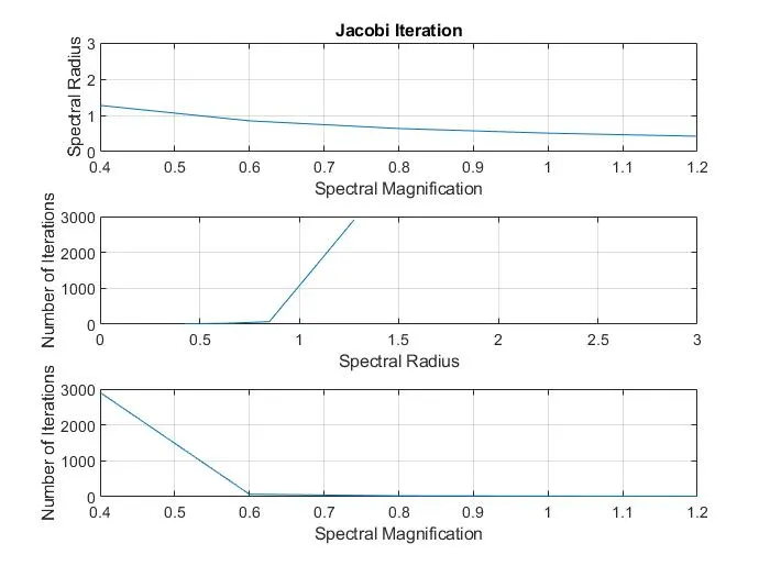
Figure 1

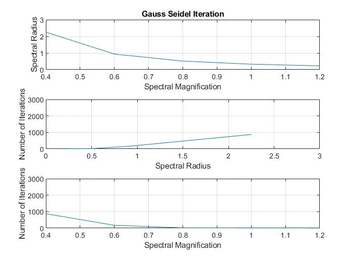
Figure 2

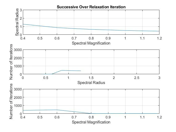
Figure 3

The graphs are all scaled to the same axis in all figures for comparison. To improve the observation results one can change the axis demarkations and compare.

CONCLUSION:

Each figure clearly depicts that As spectral magnification increases, spectral radius decreases (subplot 1) and number of iterations to converge decreases (subplot 3).

(Subplot 2) depicts that as spectral radius increases, the number of iterations to reach convergence also increases.

Observing the convergence as a function of spectral magnification, in each case the spectral radius drops into the convergence range (`rho<1`) and the number of iterations show an improvement at a magnification value around 0.6.

For higher magnification values, the spectral radius drops further and the number of iterations to reach convergence also reduces significantly.

Jacobi method is the method which consumes more time and more number of iterations to reach convergence, and a better method is Gauss Seidel and after that comes Relaxation method, which adds an increment factor to the GS method.