Simulation of Flow through a pipe in OpenFOAM
Simulation of Flow through a pipe in OpenFoam
AIM:
- Write a program in MATLAB that can generate the computational mesh automatically for any wedge angle and grading schemes (wedge angle should be less than 5 degrees).
- For a baseline mesh, show that the velocity profile matches with the Hagen poiseuille's equation.
- Show that the velocity profile is fully developed.
- Post process velocity and shear stress.
OBJECTIVES OF THE PROJECT:
- Since this is a Laminar flow profile, the basic theory and formulaes should be extracted for initial and boundary conditions of flow.
- The BlockMeshDict file is programmed using MATLAB.
- The initial and boundary conditions are input and the icoFoam simulation is run.
- The velocity profile at various distances from inlet are observed.
- The shear stress variation of fully developed flow is plotted.
GOVERNING EQUATIONS AND THEORY:
The problem statement is dictated for a laminar flow in a pipe, which includes assumptions- steady, incompressible flow, 2D solution and constant flow parameters.
FLOW THROUGH PIPES:
The laminar, steady, incompressible flow includes flow of water (assumed) through a perfectly cylindrical pipe, with three velocity compopnents as discussed in the figure:
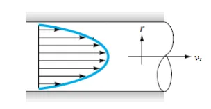
wherein `V_z` is the axial flow, `V_r` is the radial flow and `V_(theta)` is the rotational flow. The flow is governed by the continuity and the Navier-Stokes equation. Converting the equations to cylindrical polar coordinates:
`1/r(del(rV_r))/(delr)+1/r(delV_(theta))/(deltheta)+(delV_z)/(delz)=0`
For a fully developed profile, the following conditions apply: `(delV_z)/(delz)=0` and `V_(theta)=0`.
Where `mu` is the dynamic viscocity of water, `rho` is the density of water and `P` is the pressure on the center line.
Substituting them into the equation:
`1/r(del(rV_r))/(delr)=0`
and `0=-(dP)/(dx)+mu/rdel/(delr)(r(delV_z)/(delr))` (from Navier-Stokes)
Since, `P` is a function of `z` alone and `V_z` a function of `r` alone, the equation turns into,
`mu/rd/(dr)(r(dV_z)/(dr))=(dP)/(dz)=P'`
Integration of this leds to:
`V_z=(r^2P')/(4mu)+C_1lnr+C_2`
The boundary conditions input are no slip at wall: `V_z(r=R)=0` and finite velocity at `r=0`, given by `R_e=(rhoV_(avg)D)/mu`
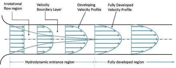
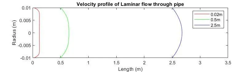
`V_z=-(P')/(4mu)(R^2-r^2)`, a parabolic shape with maximum velocity at the axis. Following is the figure demonstrating the change in velocity profile as flow becomes fully developed:
`V_(avg)=(int_0^R2pirV_zdr)/(piR^2)=-(P'R^2)/(8mu)=V_max/2`
This concludes to the pressure difference formulation by Hagen Poiseuille Law:
`P'=(dP)/dx=-(32muV_(avg))/(D^2)`
The length of the pipe is considered using: `L=0.06.R_e.D`
The problem is solved using a Laminar flow regime and the following flow property values:
`R_e=2000`
`D=0.02m`
`mu=(0.89).10^-3 Pa.s`
`rho=1000(kg)/m^3`
BODY OF THE CONTENT:
The following MATLAB code is written for the creation of BlockMesh Dict file:
CODE:
%Creating a blockmestdict file for Hagen-Poiseuille Law
clear all, close all,clc

%Flow parameters input
Re=2000;
rho=1000;
D=0.02;
R=D/2;
L=0.06*Re*D;
mu=0.00089;
nu=mu/rho;
%Wedge angle for pipe
theta=2.5;

%Boundary Conditions
v_avg=Re*nu/D;
v_max=2*v_avg;
L=L+0.3;
dp=(8*v_avg*mu*L)/R^2;

%Vertices
v0=[0 0 0];
v1=[0 R*cosd(theta/2) -R*sind(theta/2)];
v2=[0 R*cosd(theta/2) R*sind(theta/2)];
v3=[L 0 0];
v4=[L R*cosd(theta/2) -R*sind(theta/2)];
v5=[L R*cosd(theta/2) R*sind(theta/2)];

%Grading factors
grading=0.2;
b1=50;
b2=1;
b3=200;

%BlockMesh Dict File
f1=fopen('blockMeshDict.txt','w');

fprintf(f1,'/*--------------------------------*- C++ -*----------------------------------*n');
fprintf(f1,'|  =========                |                                                |n');
fprintf(f1,'|        /  F ield         | OpenFOAM: The Open Source CFD Toolbox         |n');
fprintf(f1,'|       /   O peration     | Website:  https://openfoam.org                |n');
fprintf(f1,'|      /    A nd           | Version:  8                                   |n');
fprintf(f1,'|     /     M anipulation  |                                               |n');
fprintf(f1,'*---------------------------------------------------------------------------*/n');

fprintf(f1,'FoamFilen{n');
fprintf(f1,'%16s %10sn','version','2.0;');
fprintf(f1,'%16s %12sn','format','ascii;');
fprintf(f1,'%16s %17sn','class','dictionary;');
fprintf(f1,'%16s %20sn','object','blockMeshDict;');
fprintf(f1,'}n');

fprintf(f1,'// * * * * * * * * * * * * * * * * * * * * * * * * * * * * * * * * * * * * * //n');
fprintf(f1,'convertToMeters 1;nn');
fprintf(f1,'verticesn(n');
fprintf(f1,'t(%f %f %f)n',v0);
fprintf(f1,'t(%f %f %f)n',v1);
fprintf(f1,'t(%f %f %f)n',v2);
fprintf(f1,'t(%f %f %f)n',v3);
fprintf(f1,'t(%f %f %f)n',v4);
fprintf(f1,'t(%f %f %f)n',v5);
fprintf(f1,');nn');

fprintf(f1,'blocksn(n');
fprintf(f1,'hex (0 1 2 0 3 4 5 3) (%d %d %d) simpleGrading (%d 1 1)n',b1,b2,b3,grading);
fprintf(f1,');nn');

fprintf(f1,'edgesn(n');
fprintf(f1,'t arc 1 2 (0 %d 0)n',R);
fprintf(f1,'t arc 4 5 (%d %d 0)n',L,R);
fprintf(f1,');nn');

fprintf(f1,'boundaryn(n');
fprintf(f1,'t %5snt{n','axis');
fprintf(f1,'t %13s %s;n','type','empty');
fprintf(f1,'t %14sn %18sn','faces','(');
fprintf(f1,'t t %15sn %19snn %14snn','(0 3 3 0)',');','}');

fprintf(f1,'t %5snt{n','wall');
fprintf(f1,'t %13s %s;n','type','wall');
fprintf(f1,'t %14sn %18sn','faces','(');
fprintf(f1,'t t %15sn %19snn %14snn','(2 5 4 1)',');','}');

fprintf(f1,'t %5snt{n','inlet');
fprintf(f1,'t %13s %s;n','type','patch');
fprintf(f1,'t %14sn %18sn','faces','(');
fprintf(f1,'t t %15sn %19snn %14snn','(0 2 1 0)',');','}');

fprintf(f1,'t %5snt{n','outlet');
fprintf(f1,'t %13s %s;n','type','patch');
fprintf(f1,'t %14sn %18sn','faces','(');
fprintf(f1,'t t %15sn %19snn %14snn','(3 4 5 3)',');','}');

fprintf(f1,'t %5snt{n','wedgefront');
fprintf(f1,'t %13s %sn','type','wedge');
fprintf(f1,'t %14sn %18sn','faces','(');
fprintf(f1,'t t %15sn %19snn %14snn','(0 3 5 2)',');','}');

fprintf(f1,'t %5snt{n','wedgeback');
fprintf(f1,'t %13s %s;n','type','wedge');
fprintf(f1,'t %14sn %18s;n','faces','(');
fprintf(f1,'t t %15sn %19snn %14snn','(0 1 4 3)',');','}');
fprintf(f1,');nn');

fprintf(f1,'mergePatchPairs n (n );n');
fprintf(f1,'// ************************************************************************* //');

fclose(f1);
BLOCKMESHDICT FILE:
/*--------------------------------*- C++ -*----------------------------------*
|  =========                |                                                 |
|        /  F ield         | OpenFOAM: The Open Source CFD Toolbox           |
|       /   O peration     | Website:  https://openfoam.org                  |
|      /    A nd           | Version:  8                                     |
|     /     M anipulation  |                                                 |
*---------------------------------------------------------------------------*/
FoamFile
{
         version       2.0;
          format       ascii;
           class       dictionary;
          object       blockMeshDict;
}
// * * * * * * * * * * * * * * * * * * * * * * * * * * * * * * * * * * * * * //
convertToMeters 1;

vertices
(
	(0.000000 0.000000 0.000000)
	(0.000000 0.009998 -0.000218)
	(0.000000 0.009998 0.000218)
	(2.700000 0.000000 0.000000)
	(2.700000 0.009998 -0.000218)
	(2.700000 0.009998 0.000218)
);

blocks
(
    hex (0 1 2 0 3 4 5 3) (50 1 200) simpleGrading (2.000000e-01 1 1)
);

edges
(
	 arc 1 2 (0 1.000000e-02 0)
	 arc 4 5 (2.700000e+00 1.000000e-02 0)
);

boundary
(
	  axis
	{
	          type empty;
	          faces
                  (
	 	       (0 3 3 0)
                  );

              }

	  wall
	{
	          type wall;
	          faces
                  (
	 	       (2 5 4 1)
                  );

              }

	 inlet
	{
	          type patch;
	          faces
                  (
	 	       (0 2 1 0)
                  );

              }

	 outlet
	{
	          type patch;
	          faces
                  (
	 	       (3 4 5 3)
                  );

              }

	 wedgefront
	{
	          type wedge;
	          faces
                  (
	 	       (0 3 5 2)
                  );

              }

	 wedgeback
	{
	          type wedge;
	          faces
                  (
	 	       (0 1 4 3)
                  );

              }

);

mergePatchPairs
 (
 );
// ************************************************************************* //
INITIAL CONDITIONS (PRESSURE):
/*--------------------------------*- C++ -*----------------------------------*
  =========                 |
        /  F ield         | OpenFOAM: The Open Source CFD Toolbox
       /   O peration     | Website:  https://openfoam.org
      /    A nd           | Version:  8
     /     M anipulation  |
*---------------------------------------------------------------------------*/
FoamFile
{
    version     2.0;
    format      ascii;
    class       volScalarField;
    object      p;
}
// * * * * * * * * * * * * * * * * * * * * * * * * * * * * * * * * * * * * * //

dimensions      [0 2 -2 0 0 0 0];

internalField   uniform 0;

boundaryField
{
    axis
    {
        type            empty;
    }

    inlet
    {
        type            zeroGradient;
    }

    outlet
    {
        type            fixedValue;
        value           uniform 0.0152;
    }

    wall
    {
        type            zeroGradient;
    }

    wedgefront
    {
        type            wedge;
    }

    wedgeback
    {
        type            wedge;
    }
}

// ************************************************************************* //
INITIAL CONDITIONS (VELOCITY):
/*--------------------------------*- C++ -*----------------------------------*
  =========                 |
        /  F ield         | OpenFOAM: The Open Source CFD Toolbox
       /   O peration     | Website:  https://openfoam.org
      /    A nd           | Version:  8
     /     M anipulation  |
*---------------------------------------------------------------------------*/
FoamFile
{
    version     2.0;
    format      ascii;
    class       volVectorField;
    object      U;
}
// * * * * * * * * * * * * * * * * * * * * * * * * * * * * * * * * * * * * * //

dimensions      [0 1 -1 0 0 0 0];

internalField   uniform (0.089 0 0);

boundaryField
{
    axis
    {
        type            empty;
    }

    inlet
    {
        type            fixedValue;
        value           uniform (0.089 0 0);
    }

    outlet
    {
        type            zeroGradient;
    }

    wall
    {
        type            fixedValue;
        value           uniform (0 0 0);
    }

    wedgefront
    {
        type            wedge;
    }

    wedgeback
    {
        type            wedge;
    }
}

// ************************************************************************* //
CONTROLDICT FILE:
/*--------------------------------*- C++ -*----------------------------------*
  =========                 |
        /  F ield         | OpenFOAM: The Open Source CFD Toolbox
       /   O peration     | Website:  https://openfoam.org
      /    A nd           | Version:  8
     /     M anipulation  |
*---------------------------------------------------------------------------*/
FoamFile
{
    version     2.0;
    format      ascii;
    class       dictionary;
    location    "system";
    object      controlDict;
}
// * * * * * * * * * * * * * * * * * * * * * * * * * * * * * * * * * * * * * //

application     icoFoam;

startFrom       startTime;

startTime       0;

stopAt          endTime;

endTime         50;

deltaT          0.01;

writeControl    timeStep;

writeInterval   20;

purgeWrite      0;

writeFormat     ascii;

writePrecision  6;

writeCompression off;

timeFormat      general;

timePrecision   6;

runTimeModifiable true;


// ************************************************************************* //
The icoFoam solver is run for the simulation of the incompressible flow.
OUTPUT:
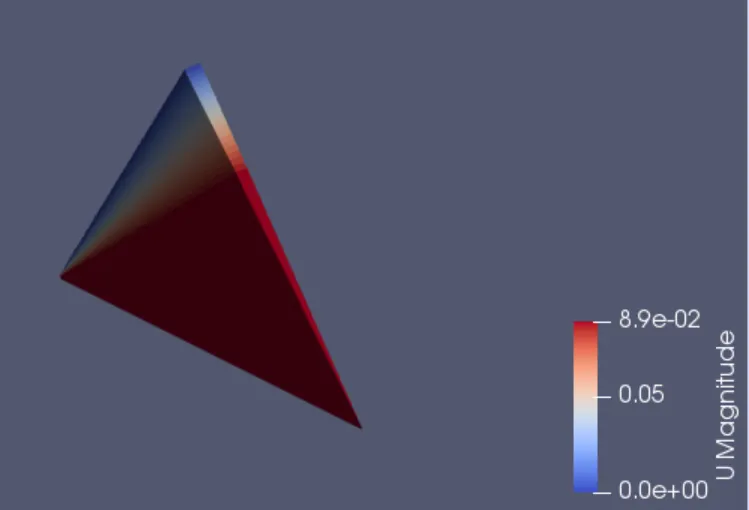
The wedge velocity profile for angle 2.5 degrees.
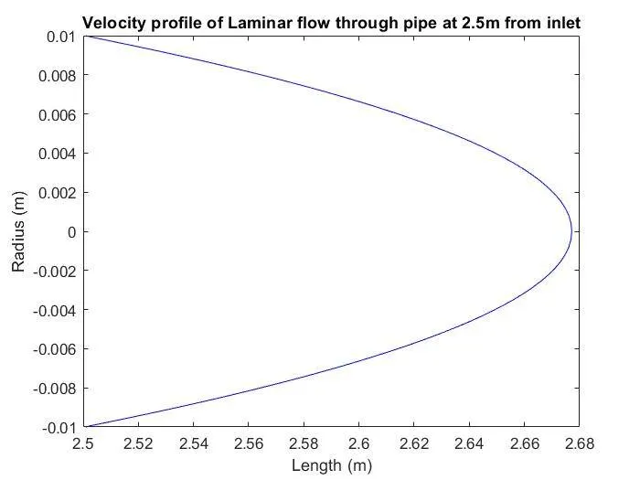
VELOCITY PROFILES AT VARIOUS LENGTHS:
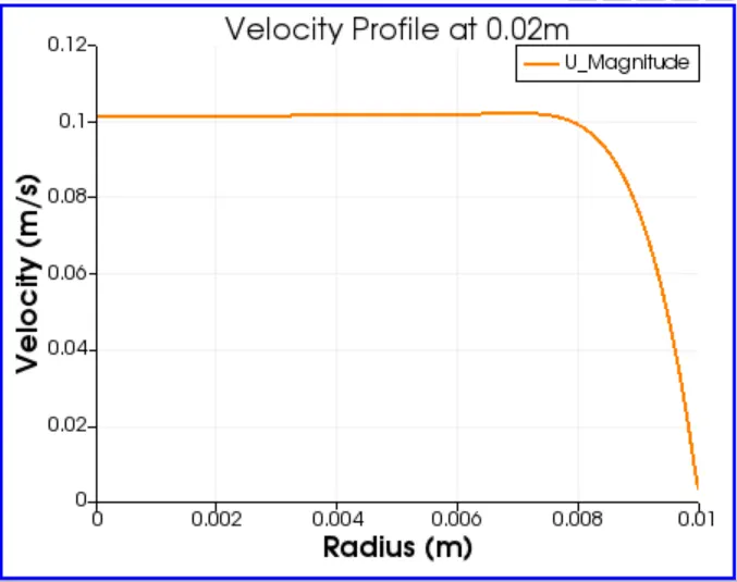
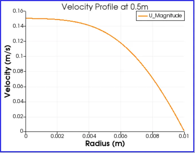
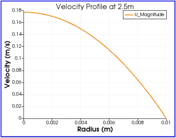
To visualize the above velocity profiles, the image should be inverted 90 degrees clockwise, and a water image of the profile should be taken. This is because the figure only represents the flow from `r=0 to r=R`, and not the whole pipe diameter. To create the whole velocity profile plot, the csv files at the three time steps are extracted and the plots are generated in MATLAB.
VELOCITY PROFILE PLOT:
%Program to extract and plot the velocity profiles at various input lengths
clear all, close all, clc
%The data is extracted from the respective csv files.
T=readtable('0.02.csv','Range','A2:A1001');
%Table format cannot be used for plotting and is converted to array
V=table2array(T);
%The radius is defined as the y-axis parameter for the pipe flow
r=linspace(0,0.01,1000);
%r2 is defined to mirror the pipe flow, for the same velocity profile in
%the lower half of the pipe.
r2=linspace(0,-0.01,1000);
figure(1)
V=V+0.02;
plot(V,r,'r')
hold on;
plot(V,r2,'r','HandleVisibility','off')

%Extraction and Plotting of velocity profile at 0.5m input length
T2=readtable('0.5.csv','Range','A2:A1001');
V2=table2array(T2);
V2=V2+0.5;
plot(V2,r,'g')
hold on;
plot(V2,r2,'g','HandleVisibility','off')

%Extraction and Plotting of velocity profile at 2.5m input length
T3=readtable('2.5.csv','Range','A2:A1001');
V3=table2array(T3);
V3=V3+2.5;
plot(V3,r,'b')
hold on;
plot(V3,r2,'b','HandleVisibility','off')
legend('0.02m','0.5m','2.5m')
axis([0 3.5 -0.01 0.01])
title('Velocity profile of Laminar flow through pipe')
xlabel('Length (m)')
ylabel('Radius (m)')
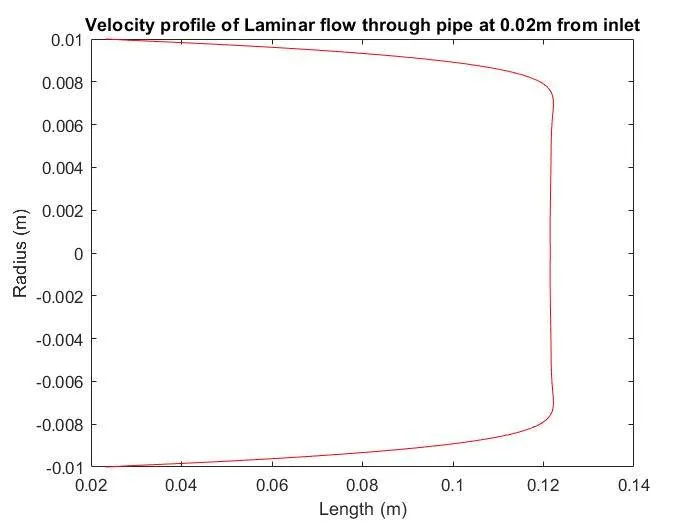
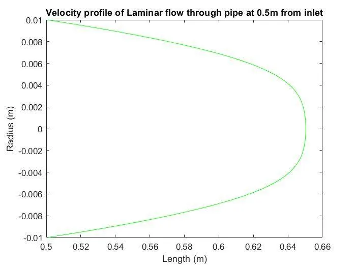
The following plots were obtained on individual analysis:
Comparing the velocity profiles in a single image:
The following code is written for the calculation and plotting of Shear stress profile:
SHEAR STRESS PROFILE PLOT:
%Shear Stress Profile plotting
clear all, close all, clc

%The radius is defined as the y-axis parameter for the pipe flow
r=linspace(0,0.01,1000);
%r2 is defined to mirror the pipe flow, for the same velocity profile in
%the lower half of the pipe.
r2=linspace(0,-0.01,1000);

%Extraction and Plotting of Shear Stress profile at 2.5m input length
T3=readtable('2.5.csv','Range','A2:A1001');
%Converting the table format data to array format
V3=table2array(T3);

%Shear Stress Profile
%Dynamic viscocity
mu=0.0089;
for i=2:length(V3)
   tau(i)=mu*((V3(i)-V3(i-1))/(r(i)-r(i-1)));
end
for i=2:length(V)
   tau2(i)=mu*((V3(i)-V3(i-1))/(r(i)-r(i-1)));
end
plot(tau,r,'r')
hold on;
plot(tau2,r2,'b')
title('Shear Stress Distribution in Pipe Flow')
xlabel('Length (m)')
ylabel('Radius (m)')
OUTPUT: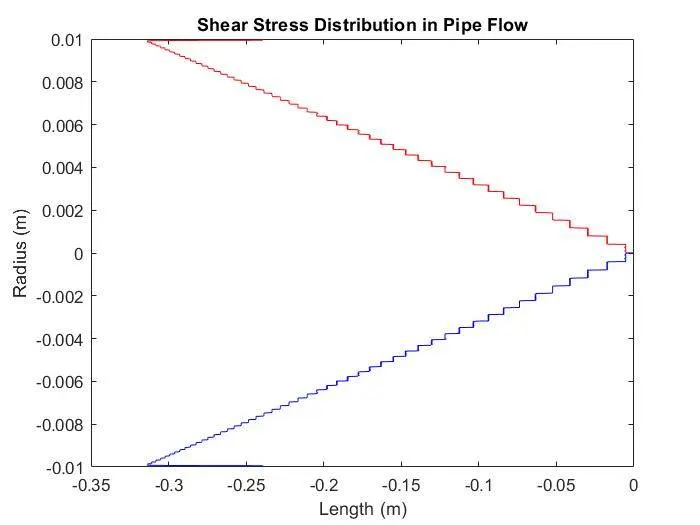
CONCLUSION:
It can be observed that the flow is developed, by comparing the velocity profile at the exit of the pipe.
The Shear Stress profile also matches literature. The steps observed in the Shear Stress profile is the cell dimension of the Fintie volume Method simulation.
The theoretical velocity at center line is obtained as 0.178 m/s and the experimental value obtained is 0.1771 m/s.