Genetic Algorithm
OPTIMIZATION OF STALAGMITE FUNCTION USING GENETIC ALGORITHM
AIM:
- Optimize the stalagmite function and obtain the global maxima using MATLAB.
THEORY:
Genetic Algorithms are an optimization technique used to solve non-linear or non-differentiable optimization problems. They use concepts from evolutionary biology to search for a global minima to an optimization problem. The name is derived from the principle of mimicking evolutionary techniques. The primary difference between a classical algorithm and genetic algorithm are:
- Classical algorithms generate a single point at each iteration. The sequence of the points approach an optimal solution. Whereas, genetic algorithm or GA generates a population of points at each iteration, and the most fit point converges to give optimal solution.
- Classical algorithms select the next point in the sequence using deterministic computation, whereas GA selects the next population by random number generator.
GA works by starting an initial generation of candidate solutions that are tested against the fitness function. This then generates subsequent generations of points from the first generation using the step-wise processes of Selection, Crossover and Mutation.
Fitness function is a function which designates a fitness candidate value for each candidate in the workspace. The 1st step involves assigning the candidates their respective fitness value. The most fit candidate for the function has a higher chance of getting selected for the next stage and has higher chances of creating clones for the next data set. After the parent generation is selected at random, crossover of these candidates takes place. Crossover refers to random pairing of candidates to observe a mixed characteristic in the child generation of candidates. After crossover of the parent candidates, in the new generation of the child candidates a random characteristic is introduced in one/few candidates. This is done to introduce all possibilities of the evolution algorithm devised. After the mutation process, the child candidates are again assigned fitness values using the fitness function. The iteration is stopped when the algorithm observes that very minimal change or no change is observed in the subsequent child candidates when compared to the parents.
ANSWERS TO QUESTIONS:
- Stopping Criteria: A stopping criteria can be coded into the loop. After every GA iteration, the optimal solution values can be compared to the previous iteration’s solutions. If the standard deviation is zero or of minimal acceptable tolerance, the ‘break’ command can be used to exit the loop. This is done because further iterations can lead to the same solutions while consuming lot of time.
- Syntax: Mentioned below are the syntax of the ‘ga’ function used:
[xval,fval]=ga(@func,nval);_____(1)
where ‘func’ refers to the function to be optimized, ‘nval’ refers to the number of dimensions in which the position of minima is desired, ‘fval’ refers to the function value at the optimized global minima, and ‘xval’ is a vector which stores the position of global minima based on ‘nval’ value.
[xval,fval]=ga(@func,nval,A,b,Aeq,beq,lb,ub); _____(2)
where ‘A’ and ‘b’ represent any linear inequalities for the optimization- (A*x<=b). Similarly, ‘Aeq’ and ‘beq’ are linear equality conditions for optimization- (Aeq*x=beq). Here ‘lb’ and ‘ub’ represent set of lower bound and upper bound respectively, on the design variables to formulate the solution is the range (lb<=xval<=ub).
[xval,fval]=ga(@func,nval,A,b,Aeq,beq,lb,ub,nonlcon,IntCon,options); _____(3)
subjects the minimization of the constraints defined in ‘nonlcon’. The function ‘nonlcon’ accepts ‘xval’ and returns vectors C and Ceq, representing the nonlinear inequalities and equalities respectively. ga minimizes the fun such that (C(x) ≤ 0 and Ceq(x) = 0). The above function avails the variables listed in ‘IntCon’ take integer values. The ‘options’ syntax is used to vary the default optimization parameters by the values stated in ‘options’.
options=optimoptions(SolverName,Name,Value); _____(4)
return a set of default options for the ‘SolverName’ solver, for the ‘Name’ parameter, altered with the specified ‘Value’.
- Significance of running multiple iterations: Each iteration refers to a new generation of candidates created after crossover and mutation. The fitness values of the new candidates are fund using the fitness function, and on the top ‘k’ fit candidates of the new generation are replaced with the bottom ‘k’ fit candidates of the parent generation. Therefore, higher number of iterations lead to more generations of candidates where all types of characteristics are available and more accurate solution is found based on the fitness values. When the algorithm starts, the initial parent population is randomly selected by the ga solver. The subsequent generations of crossover and mutation lead to convergence at the global minima solution. Hence, lower number of iterations will lead to a solution closer to the randomly selected parent population.
- Case Studies:
Study 1 refers to a Statistical analysis to for the optimization of the global maxima. Eqn.1 will be used to select a random population of candidates and run the program till the solution converges. This study involves using ga to provide an optimal solution, but when the function values are plotted as a against number of iterations, a lot of scattering is observed. This is occurring mainly because of a large space set from which the algorithm is choosing the parent population. To constrict the available space for the algorithm, the next case study is applied.
Study 2 refers to the similar Statistical analysis with upper and lower bound limits. Eqn.2 will be used for this computation. No linear equalities or inequalities are input for this study, therefore A,b,Aeq,beq would be a null set [] input in the equation. The algorithm puts limits on the selection algorithm of ga. The parent population is only selected from the specified, constricted zone mentioned by the user. Therefore, for a given number of iterations the algorithm is improved to provide much fitter generations in much less iterations. But when the output will be observed there will be a dip at 2 points, still providing a confusing output of maxima. The number of iterations provided by the user to run the loop is not linked to the number of iterations ga internally does to give the most fit results. To understand this the next study is performed.
Study 3 refers to the Statistical Analysis with upper and lower bound limits and a higher number of iterations per ga cycle. Eqn.3 will be used for the computation of this case. No input on the nonlcon and IntCon is specified, therefore they will be left as null sets []. Input will be provided in options function discussed in Eqn.4. The formula mentioned would be used to improve the population index of the ga cycle to 200. The best optimization is observed in this case study as with a constricted upper and lower bounds the parent population is wisely chosen (even though random). And the increased number of iterations per cycle on the loop for ga, ensures that the more generations of child populations are created and the candidates with best fit is found for the solution.
GOVERNING EQUATIONS:
Stalagmite Function:
The genetic algorithm solver in this study is used to optimize the stalagmite function. The function is stated below:
`f(x,y)=f_(1,x).f_(2,x).f_(1,y).f_(2,y)` _____(5)
where:
`f_(1,x)=[sin(5.1πx+0.5)]^6`
`f_(1,y)=[sin(5.1πy+0.5)]^6`
`f_(2,x)=exp[−4ln(2)(x−0.0667)^2/0.64]`
`f_(2,y)=exp[−4ln(2)(y−0.0667)^2/0.64]`
It should be noted that, when we multiply all the parameters for `f(x,y)`, a negative sign must be used. This inverts the function, and the ga solver actually finds the coordinates of the global maxima.
OBJECTIVES OF THE PROJECT:
- Firstly, a domain is created for the stalagmite function. And the stalagmite function is computed for each x and y value. A negative sign is used in the stalagmite function to ensure that the whole plot is reversed. Therefore, applying the ga solver on this function gives out the global minima, which is actually the global maxima.
- This dataset is applied to each case study in the ga solver mentioned above with the respective limits and population size values.
- The dataset is plotted with the optimized solution to observed the variation of results in each case.
BODY OF THE CONTENT:
CODE EXPLAINATION:
Firstly, a data space in created using linspace command for x and y.
The meshgrid command is used to create a 2D grid for the formulated x and y values. This is input in xx and yy, as a 2D matrix to store the grid values of each locations x and y coordinates.
A loop is run over each xx and yy grid point to compute the stalagmite function and the output is saved in ‘f’.
For Case 1, a loop is run over a specified case iterations and Eqn.1 is used to obtain the optimized solution. The solution’s x and y coordinate is stored in xopt and yopt, and the function value is stored in fopt.
For plotting, a single figure is used with 2 subplots. The 1st subplot includes a surfc command to plot the surface (xx,yy,-f). ‘-f’ is used to create the original stalagmite plot. The results obtained in the xopt,yopt and fopt are plotted in the same subplot of figure. Again, the ‘-fopt’ is used to invert the originally inverted stalagmite function.
In the 2nd subplot of the figure, the fopt value is plotted against the iteration number. This is done to observe the discrepancies in each case, as a function of number of iterations.
Similarly, for each case study the respective case equations are used to optimize the stalagmite function and plot the results.
CODE:
clear all, close all, clc
%Optimization of Stalagmite Function using Genetic Algorithm
%Initially a dataset is created, from which the function is formulated
%linspace command is used to create data values for x and y
x=linspace(0,0.6,150);
y=linspace(0,0.6,150);
%number of test cases is taken as 50
num_cases=50;
%meshgrid command is used to plot the x and y data values on a 2D grid, and
%create a 2D array of thr plot with x and y coordinates
[xx,yy]=meshgrid(x,y);
%a loop is run for each value of xx and yy n the meshgrid. And the
%stalagmite function is called for each vale. This creates the function
%value f at each point on the 2D mesh grid.
for i=1:length(xx)
    for j=1:length(yy)
        input(1)=xx(i,j);
        input(2)=yy(i,j);
        f(i,j)=stalagmite(input);
    end
end

%Study 1: Statistical Behaviour
%Firstly, a loop is run for each crossover and mutation of the candidates
%inputs1 stores the local minima (x,y) given out after the 1st cycle.
%And the fopt1 stores the function value at each cycle point.
%ga(function,value) is used to compute the algorithm for the 'function; and
%output 'value' dimensioned optimized points
for i=1:num_cases
    [inputs1, fopt1(i)]=ga(@stalagmite,2);
    xopt1(i)=inputs1(1);
    yopt1(i)=inputs1(2);
end
%Figure is created with a subplot 2x1, where the 1st image described is the
%surfc and plot3 command.
%surfc plots a 3D surface of the dataset required.
figure(1)
subplot(2,1,1)
hold on
%-f is used as in the stalagmite function, negative sign was added to find
%the local maxima. Hence to observe the original plot,'-f' is used.
surfc(xx,yy,-f)
%shading interp removes the gridlines from the surface plot
shading interp
%plot3 command is used to plot the solution vectors, i.e. x,y and z
%coordinates of the optimized solution
plot3(xopt1,yopt1,-fopt1,'marker','o','markerfacecolor','r')
title('Statistical Behaviour')
%The below subplot refers to 2nd plot in the same figure
subplot(2,1,2)
%The function values of the optimized solutions are compared, to check the
%maxima
plot(-fopt1)
xlabel('Iterations')
ylabel('Function Value')
%Study 2: Statistical Behaviour with upper and lower bounds
%Similar procedure is used as above, but in this Study lower and upper
%bound limits are input. The four [] symbols refer to input of no inequality
%and equality constraints on the x and y cooridnates.
%The set [0;0] and [1;1] define the region where the initial selection of
%the parent candidates in done. Hence, optimizing the solution and running
%the algorithm in a confined zone
for i=1:num_cases
    [inputs2, fopt2(i)]=ga(@stalagmite,2,[],[],[],[],[0;0],[1;1]);
    xopt2(i)=inputs2(1);
    yopt2(i)=inputs2(2);
end

figure(2)
subplot(2,1,1)
hold on
surfc(xx,yy,-f)
shading interp
plot3(xopt2,yopt2,-fopt2,'marker','o','markerfacecolor','r')
title('Statistical Behaviour with upper and lower bounds')
subplot(2,1,2)
plot(-fopt2)
xlabel('Iterations')
ylabel('Function Value')

%Study 3: Statistical Behaviour with increased number of iterations
%Adding to the Study 2 optimization, in this case the number of iterations
%are increased.
%optimoptions(SolverName,Name,Value) returns a set of default options for
%the 'SolverName' solver with the 'Name' parameters altered with the
%specified 'Value'
options=optimoptions('ga')
options=optimoptions(options,'populationsize',200)
%options is input into the ga function and the extra brackets after
%lower and upper bounds represent nonlcon and Intcon. The function subjects
%the minimization constraints defined in nonlcon and Intcon is defined to
%represent variables defined in Intcon as integers
for i=1:num_cases
    [inputs3, fopt3(i)]=ga(@stalagmite,2,[],[],[],[],[0;0],[1;1],[],[],options);
    xopt3(i)=inputs3(1);
    yopt3(i)=inputs3(2);
end

figure(3)
subplot(2,1,1)
hold on
surfc(xx,yy,-f)
shading interp
plot3(xopt3,yopt3,-fopt3,'marker','o','markerfacecolor','r')
title('Statistical Behaviour with increased number of iterations')
subplot(2,1,2)
plot(-fopt3)
xlabel('Iterations')
ylabel('Function Value')
STALAGMITE FUNCTION CODE:
%function to compute negative of stalagmite function values
function [f]=stalagmite(input_vector)
   %input_vector contains 2 values which are designated to x and y
   %respectively
   x=input_vector(1);
   y=input_vector(2);
   %each term is formulated and multiplied
   term1=(sin(5.1*pi.*x+0.5)).^6;
   term2=(sin(5.1*pi.*y+0.5)).^6;
   term3=exp((-4*log(2)).*((x-0.0667).^2)./0.64);
   term4=exp((-4*log(2)).*((y-0.0667).^2)./0.64);
   %negative value is used, so as to formulate the global maxima using ga
   %solver
   f=-(term1.*term2.*term3.*term4);
end
OUTPUT:
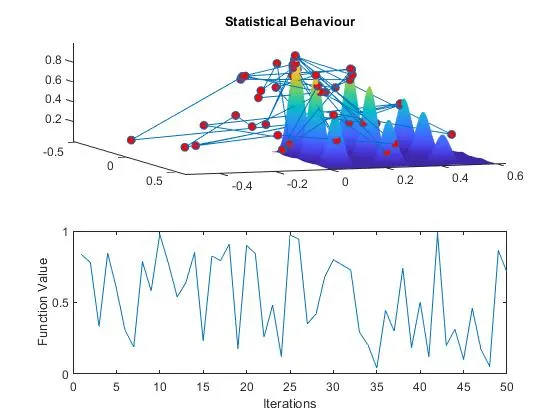
Figure 1
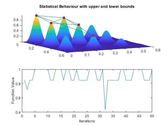
Figure 2
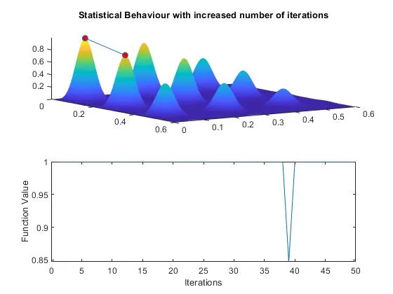
Figure 3
- No errors were encountered during the code execution.
RESULTS AND CONCLUSIONS:
- In Case 1, the Statistical Behaviour of the ga solver shows a highly scattered dataset of points. The highlighted points in Subplot 1 of Fig.1, which are nowhere near the surface of the stalagmite plot, are the initial generations of the population, which are chosen at random. The function value in the Subplot 2 show high scattering. This method for optimization does not provide an accurate global maxima for the stalagmite function.
- In Case 2, the Statistical Behaviour with upper and lower bounds on the ga solver workspace shows some rectification of the scattering. The Subplot 1 of Fig.2 shows that most of the highlighted points are near to the surface of stalagmite plot, and clearly prove that they converge to the global maxima. This is happening because of the limits input into the ga solver. The random selection of the initial generation (parent) is done only in the specified zone. Therefore, lower discrepancies are observed in the Subplot 2 of Fig.2. The two dips observed in the Subplot 2 still show that more iterations are required to finalize the most fit candidate among the shortlisted ones.
- In Case 3, the increase in iteration number or the population size of the ga solver shows a lot of improvement in the Statistical Behaviour. In the Subplot 1 of the Fig.3, the highlighted points clearly show minimum scattering, and one solution of the global maxima. The increased number of iterations shows a single optimized solution in the Subplot 2 of function values. This case combines the reduced working space of ga solver with the increased iteration number, to select the most fit candidate(point) for the global maxima.
REFERENCES: