CFD Simulation comparing mixing efficiency at a Tee-junction using ANSYS Fluent
MIXING EFFICIENCY:
AIM:
To run a CFD Steady state simulation for a Tee Mixing problem for hot inlet velocity=`3 text( m/s)` and temperature= `36^0 C`, and cold inlet temperature= `19^0C`. The simulation is run for two case bodies of various lengths and two momentum ratio-2 and 4.
OBJECTIVES OF THE PROJECT:
Expected Results to be plotted:
- Velocity and temperature contour plots on the cut planes along and across the pipe.
- Velocity and temperature line plots along and across the length of the pipe.
- Perform Mesh independent study for any one case.
- Discuss the effect of length and momentum ratio on results.
INTRODUCTION:
The problem statement involves mixing of two fluids (air) in a Tee Junction pipe flow at different temperatures and velocities. The simulation is run to observe the variation in results for various turbulence models and lengths of the outlet pipe. Turbulent mixing of fluids of different temperatures in T-junction geometries are important in the field of nuclear reactor safety. High transient temperature fluctuations at adjacent pipe walls, cyclic thermal stresses and fatigue are few important domains of analysis. Other applications of T-mixing include:wastewater managment to petroleum oil transmission to any branch dealing with fluids. A T-junction invloves mixing of fluids at right angles, wherein one fluid is along the mainstram path and an additional input joint is added to this flow.
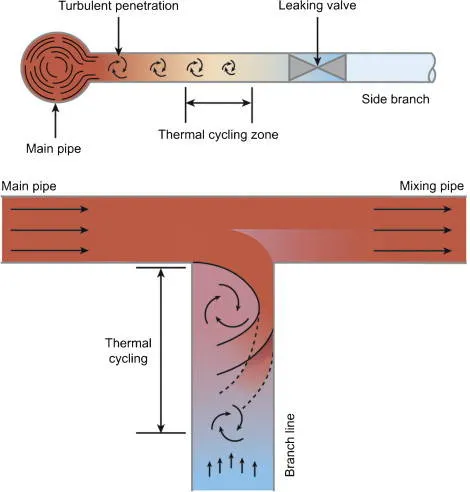
Fig. 1 Tee-junction layout
Understanding the simulation and its application is very critical while dealing with fluids in nuclear reactors and petroleum pipelines. Turbulent fluid mixing invloves vortex shedding, velocity fluctutations, and whirls. Dealing with the respective fluids in these conditions or designing a flow and mixing mechanism to avoid such intricacies needs a pre-hand CFD simulation to understand the flow.
GOVERNING EQUATIONS AND THEORY:
Mixing of two fluids or in general any fluid mechanics flow need to follow the basic mass conservation, momentum conservation and energy conservation equations (Navier Stokes Equations). For the derivation of theoretical enthalpy and temperature of the mixed flow the following formulaes are used:
`T_(mixture)=(m_(hot)T_(hot)+m_(cold)T_(cold))/(m_(hot)+m_(cold))`
`h_(mixture)=(m_(hot)h_(hot)+m_(cold)h_(cold))/(m_(hot)+m_(cold))`
where `m` is the mass flow rate and `h` is the enthalpy of the respective flows.
MODELLING:
The turbulence models employed for comparison are:
Realizable `k-epsilon` model: It is a two equation model that gives a general description of turbulence by means of two transport eqations (PDEs). The first transported variable is the turbulent kinetic energy (k). The second transported variable is the rate of dissipation of turbulent kinetic energy (ε). k-ε model focuses on the mechanisms that affect the turbulent kinetic energy. The mixing length model lacks this kind of generality. The underlying assumption of this model is that the turbulent viscosity is isotropic, in other words, the ratio between Reynolds and mean rate of deformation is the same in all directions.
`k-omega` SST model: The k–omega (k–ω) turbulence model is a common two-equation turbulence model, that is used as an approximation for the Reynolds- Averaged Navier Stokes (RANS equations). The model attempts to predict turbulence by two PDEs for two variables, k and ω, with the first variable being the turbulence kinetic energy (k) while the second (ω) is the specific rate of dissipation (of the turbulence kinetic energy k into internal thermal energy).
SOLVING APPROACH:
For solving the problem statement, the following flow chart is followed:
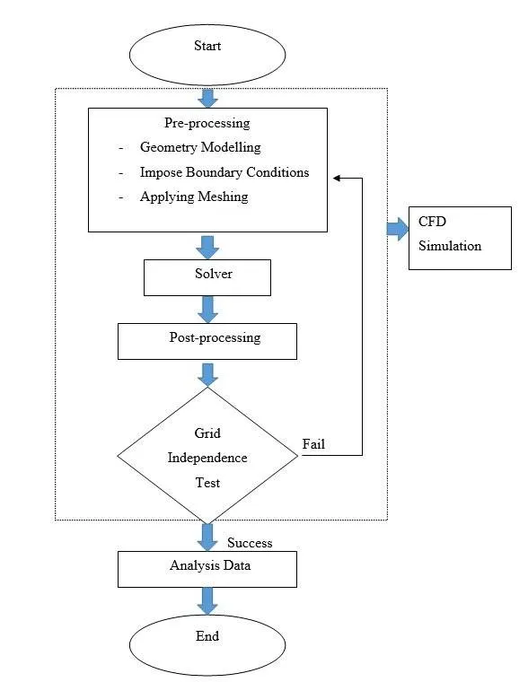
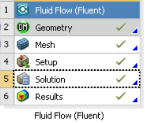
Fig. 2 ANSYS Solving Flow Chart
ANSYS involves selection of Fluent solver, input and verification of Geometry, Meshing, Setup, Solutions and Results. The Geometry is input in ANSYS Space Claim. The mesh sizing and face naming is done while Meshing. The Setup section involves Mesh Checking, Turbulence Model selection, Solver type, velocity formulation and time (steady or transient state), Output report files, Material selection, Initial and Boundary conditions. The Results section is used for the visualiztion of the output in a GUI.
PRE-PROCESSOR AND SOLVER SETUP:
The problem statement includes a hot air of `36^0C` input from the larger diameter inlet at speed 3m/s and cold air of `19^0C` input from the smaller diameter inlet. The pressure at the outlet end is set at atmospheric pressure. The Momentum Ratio is defined as:
`text(Momentum Ratio) (MR)= (text(Velocity of cold inlet))/(text(Velocity of hot inlet))`
For each geometry length, the MR has two case values 2 and 4.
GEOMETRY:
The pre-processor involves Geometry and Mesh Setup. The Geometry tab is opened in the Fluent Palette. A pre-modeled CAD model is input. The model is actually the model of the T-junction pipe. Therefore, a Volume Extract is to be created which will later be filled with the respective fluid for simulation. The volume is extracted using the 3 faces (2 inlet, 1 outlet). The solid pipe section is hidden or "Suppressed for Physics", which only takes only the volume extract for simulation. This window is closed as the geometry is automatically saved.
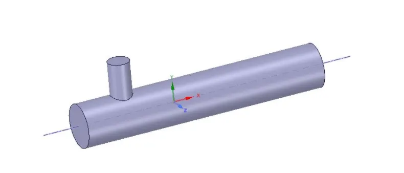
Fig. 3 Geometry for simulation
MESH:
The Mesh tab is opened from the Fluent Pelette. Face Selection is used to name the respective inlet and outlet faces. Mesh section is selected and in the details the element size is set to `1e^(-3)`. Generate Mesh is selected for the mesh to be computed. Since the pipe section is symmetrical, a symmetry plane can be introduced to reduce the computation time. New Section Plane is selected and a line is drawn along the axis of the main pipe. The following meshed figure is obtained for further computation:
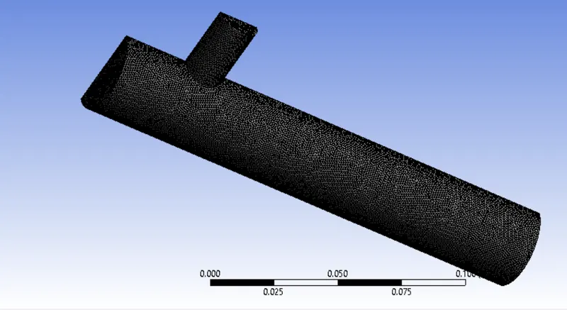
Fig. 4 Meshed geometry
In the Mesh Details, Quality parameter is defined. In its Mesh Metric, the Element Quality can be guaged. For the above figure the following mesh element quality is obtained:
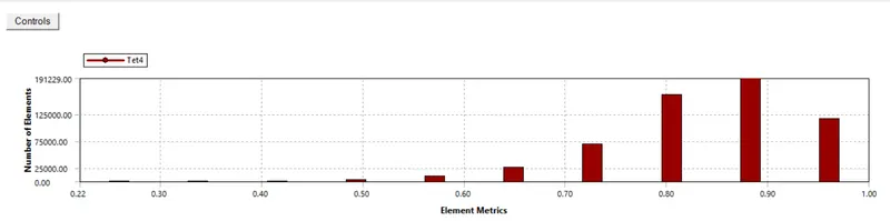
Fig. 5 Element Quality Metrics
The minimum acceptable Metric is 5%. The lowest for this mesh is 22%, therefore the computation can be continued.
SETUP:
In the Domain section, a Check Mesh option is available to verify if the Mesh has loaded properly for initializing other conditions. If the Mesh is perfect, the Console gives a positive feedback. The Physics section includes the general solver details. Here the Steady state, Pressure based, Absolute Velocity solver is selected. For the temperature computations Energy is ticked off, to be included in the equations. The Viscous section is opened as a turbulent model is to input for the simulation. Here based on the simulation, a `k-epsilon text( Realizable)or k-omega text( SST)` model is selected. Add Materials option is selected for selecting the fluid for the flow, which is air. In the Zones bar, Boundaries section is selected for input of boundary conditions. Each boundary is selected and the respective velocity and temperature values are input.The outlet face is also selected and atmospheric pressure (1atm) is input. In Solving section, in Definitions, New, Surface Reports- Area weighted Average and Standard Deviation Reports are selected for both velocity and temperature at the outlet face. The solver is initialized to t=0, and Hybrid Initialization is selected. The number of iterations is input and the Calculate button is selected to start the simulation.
Once the simulation is completed, if the solution has converged, the console shows the statement for convergence. If not, it is recommended to run the simulation for more iterations, or if the residual chart in the Graphics section shows a stable graph for each parameter, convergence can be expected. The system doesn't show the Convergence statement as a tolerance value of `1e^(-6)`is set. Residuals are basically the difference between the exact solution and the system's numerical solution.
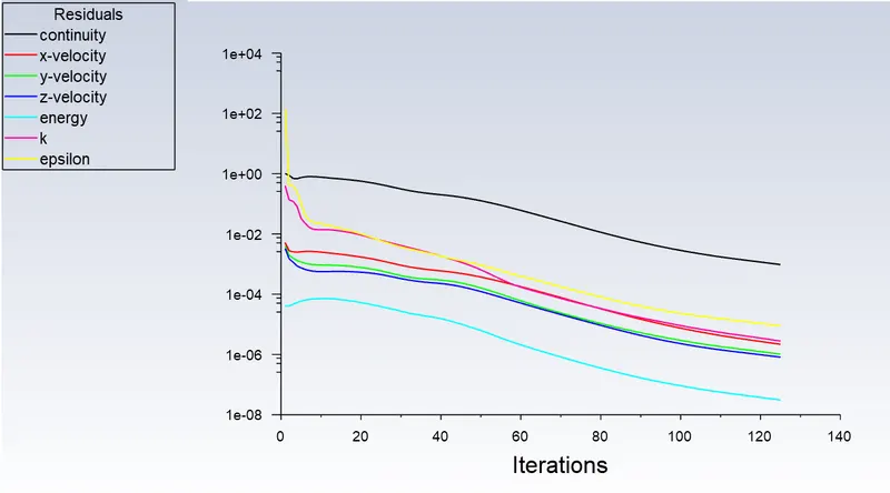
Fig. 6 Residuals variation as a function of iteration number
Similar plots for the Area weughted Average and Standard Deviation values of velocity and temperature are plotted parallelly. The Fluent Setup is closed, and the results are automatically saved.
RESULTS:
The Results tab in the Fluent Palette is opened. Using the Insert option various planes and lines are drawn to access the variation of output parameters along the geometry. The respective plane's color is selected to Variable, and the variable is selected as velocity or temperature based on the desired output.
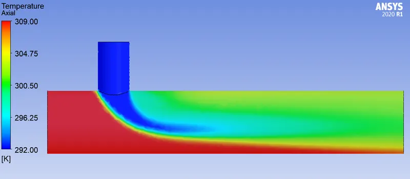
Fig. 7 Axial Plane Temperature Variation
OUTPUT:
GRID DEPENDENCE TEST:
The Mesh Dependence study was performed for the Momentum Ratio `MR=2`, short length pipe. The two mesh element sizes considered were `5e^(-3)` and `1e^(-3)`. The comparison was done for the turbulence model `k-epsilon`, and the solutions are compared at convergence. The following tabulated data shows all the comarisons:
Table 1 Mesh Grid Dependence Test
| Mesh Size | `5e^(-3)` | `1e^(-3)` |
| Tetrahedral Cell Count | 3641 | 574194 |
| Number of Iterations | 217 | 125 |
| Standard Deviation for Velocity | 0.439 m/s | 0.762 m/s |
| Area weighted Average Velocity | 4.502 m/s | 4.514 m/s |
| Standard Deviation for Temperature | 1.627 K | 1.921 K |
| Area weighted Average Temperature | 303.215 K | 303.407 K |
The theoretical outlet temperature and velocity are 303.33K and 4.5 m/s. A finer mesh is giving more accurate results for the outlet temperature value. Since the values are very close , the temperature variation plots are compared for better judgement.
Observing the axial temperature variation for both the meshing:
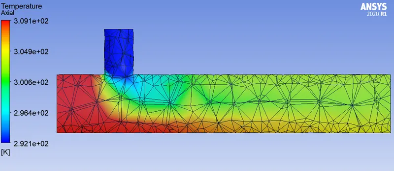
Fig. 8 Axial Plane Temperature Variation for element size=`5e^(-3)`
Fig. 9 Axial Plane Temperature Variation for element size=`1e^(-3)`
Even though the standard deviation and outlet flow variable values are similar in both cases, the refined mesh quality gives a better portrayal of temperature variation at the Tee-junction.
TURBULENCE MODEL COMPARISON:
The comparison between the `k-epsilon` and `k-omega` model was done to observe the variation in results. The comparison was done for mesh element size `1e^(-3)`, for Momentum Ratio `MR=4` Short pipe geometry. The following tabulations were made:
Table 2 Turbulence Model Comaprison
| Turbulence Model | `k-epsilon` | `k-omega` |
| Number of Iterations | 191 | 300 |
| Standard Deviation for Velocity | 0.7144 m/s | 1.128 m/s |
| Area weighted Average Velocity | 6.055 m/s | 6.1093 m/s |
| Standard Deviation for Temperature | 1.334 K | 1.812 K |
| Area weighted Average Temperature | 300.551 K | 300.704 K |
The theoretical outlet velocity and temperature for `MR=4` is 6 m/s and 300.5 K. Clearly the results for `k-epsilon` model are closer to the theoretical solution. It should be added that the `k-omega` model did not show convergence, and hence a higher number of iterations might show accepyable results. The results for `k-omega` model was considered as the Residuals chart showed a steady value over the mentioned iteration period.
All the below computations are results of `text(Realizable ) k-epsilon` turbulence model and mesh element size of `1e^(-3)`.
CASE 1: SHORT LENGTH GEOMETRY
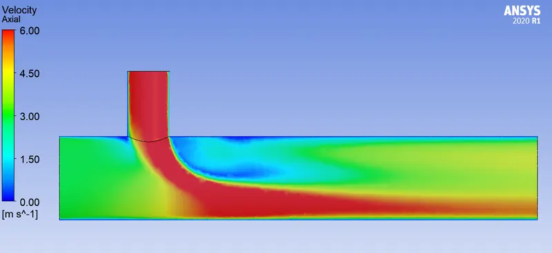
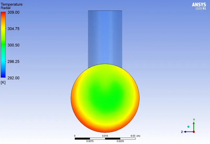
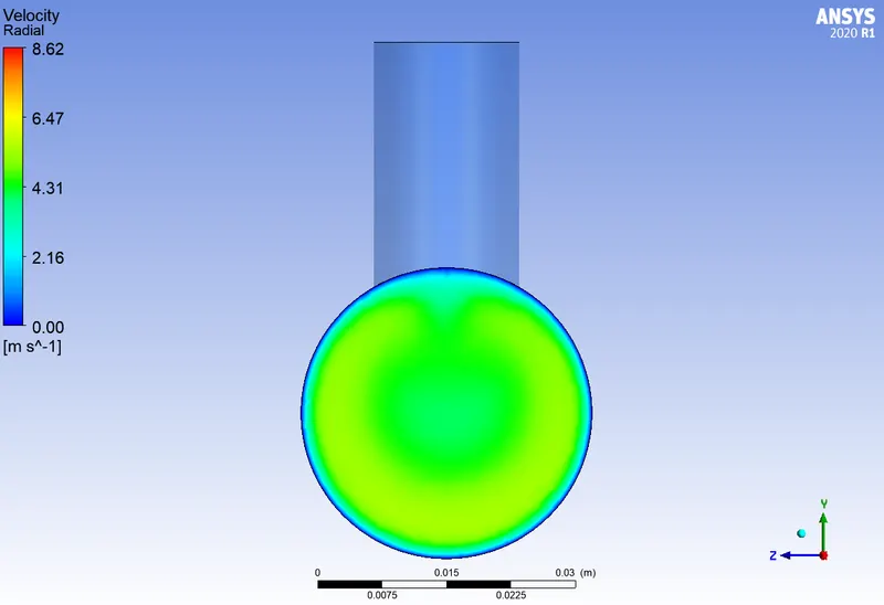
Momentum Ratio:2
(a) (b)
(c) (d)
Fig. 10 (a) Axial Plane Temperature Variation (b) Axial Plane Velocity Variation (c) Radial Plane Temperature Variation (outlet) (d) Radial Plane Velocity Variation (outlet)
(a) (b)
(c) (d)
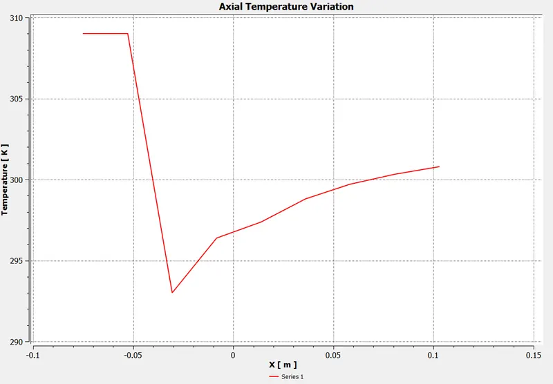
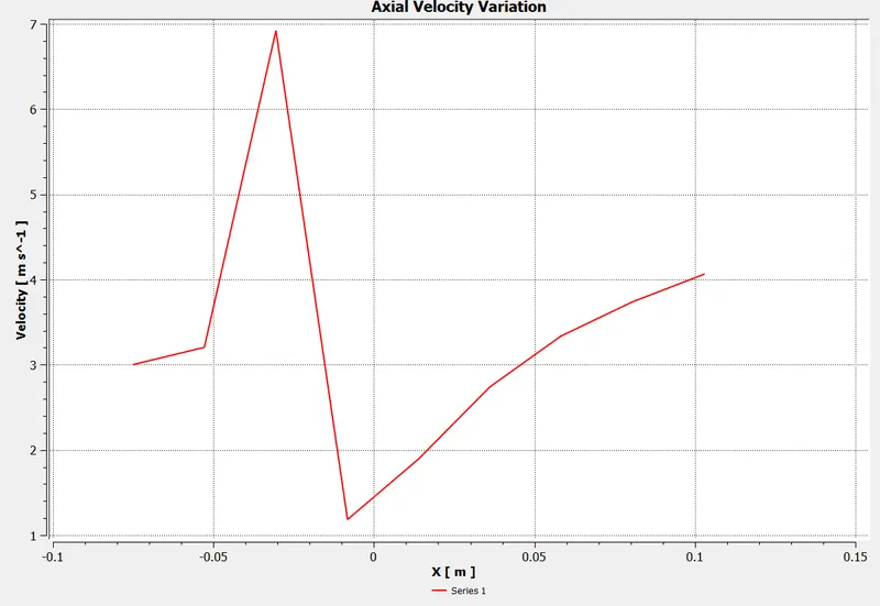
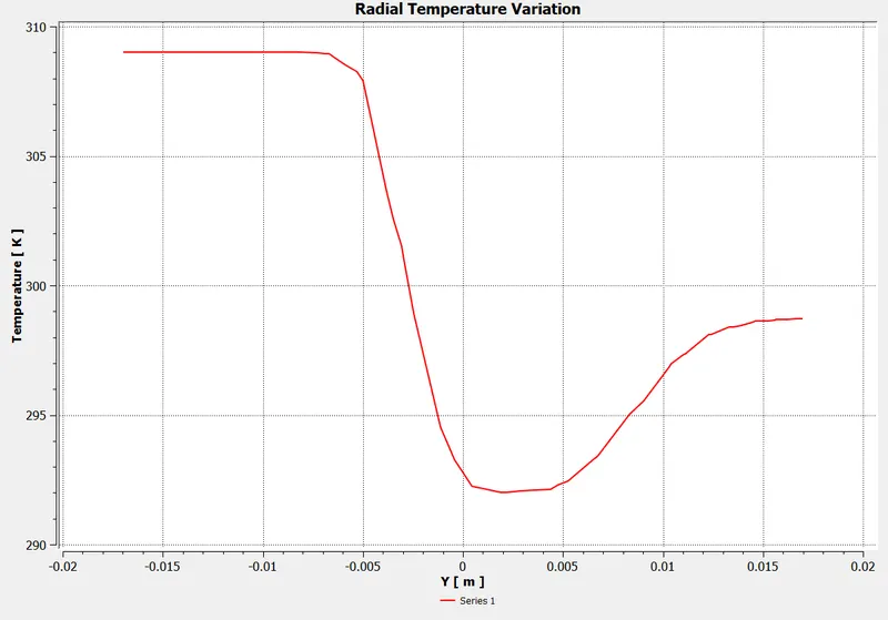
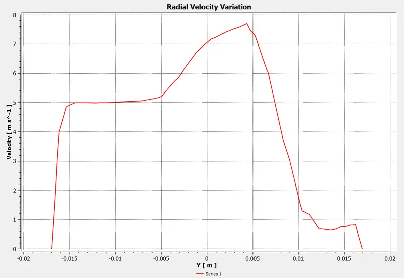
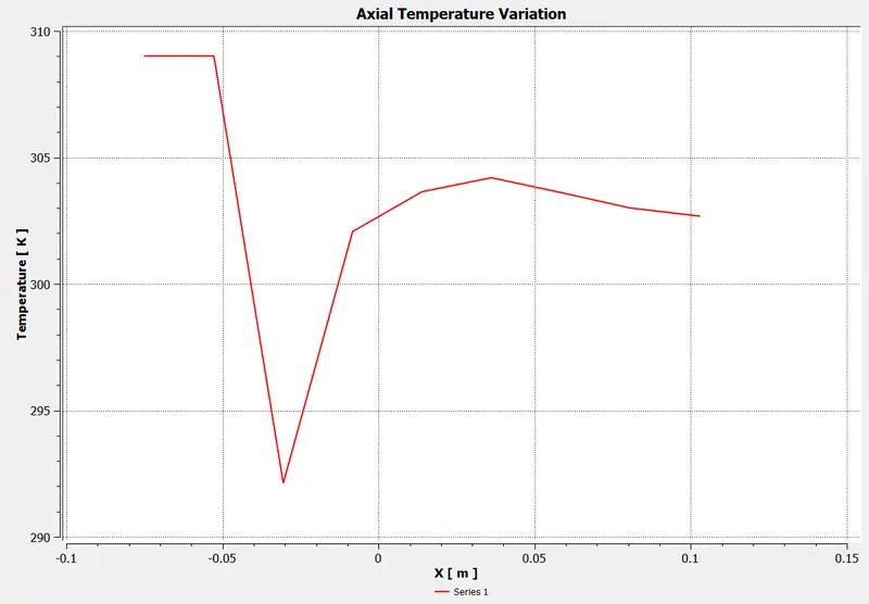
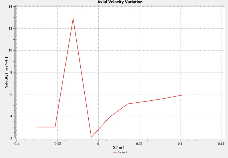
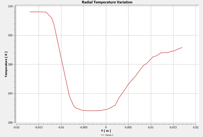
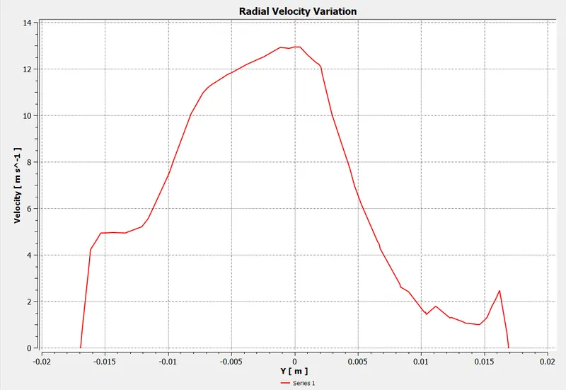
Fig. 11 (a)Temperature Variation along axis (b)Velocity Variation along axis (c)Temperature Variation along Radius (just after Tee-junction) (d)Velocity Variation along Radius (just after Tee-junction)
Momentum Ratio:4
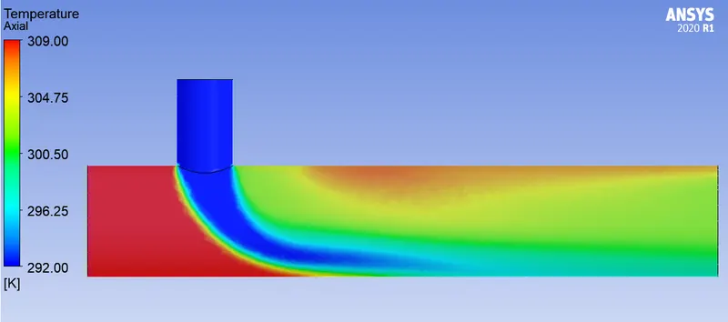
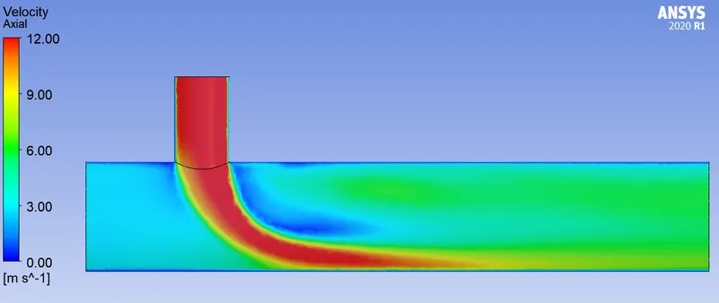
(a) (b)
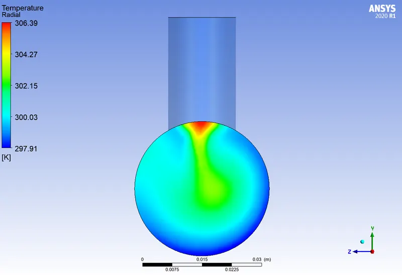
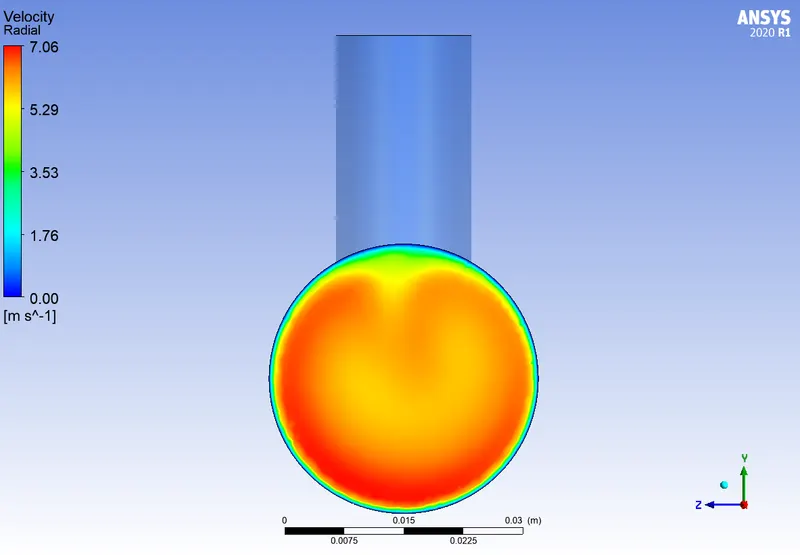
(c) (d)
Fig. 12 (a) Axial Plane Temperature Variation (b) Axial Plane Velocity Variation (c) Radial Plane Temperature Variation (outlet) (d) Radial Plane Velocity Variation (outlet)
(a) (b)
(c) (d)
Fig. 13 (a)Temperature Variation along axis (b)Velocity Variation along axis (c)Temperature Variation along Radius (just after Tee-junction) (d)Velocity Variation along Radius (just after Tee-junction)
CASE 2: LONG LENGTH GEOMETRY
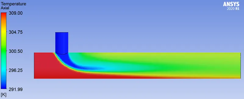
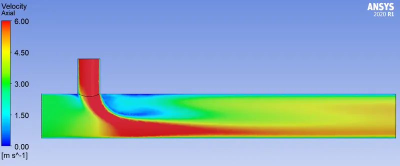
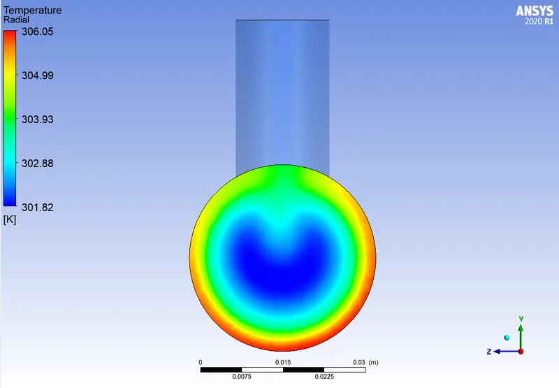
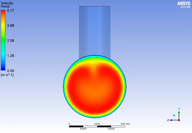
Momentum Ratio:2
(a) (b)
(c) (d)
Fig. 14 (a) Axial Plane Temperature Variation (b) Axial Plane Velocity Variation (c) Radial Plane Temperature Variation (outlet) (d) Radial Plane Velocity Variation (outlet)
(a) (b)
(c) (d)
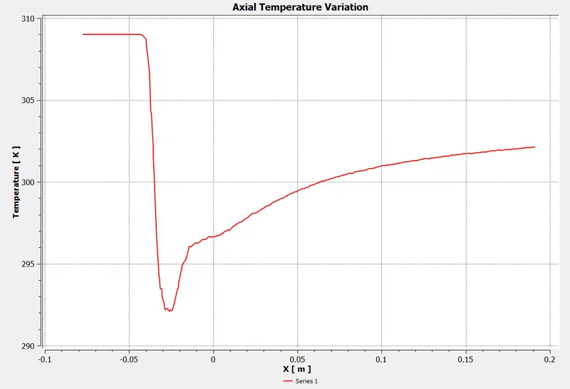
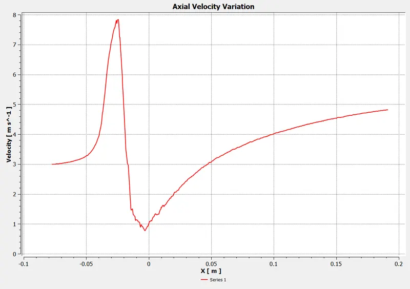
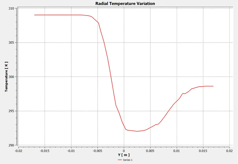
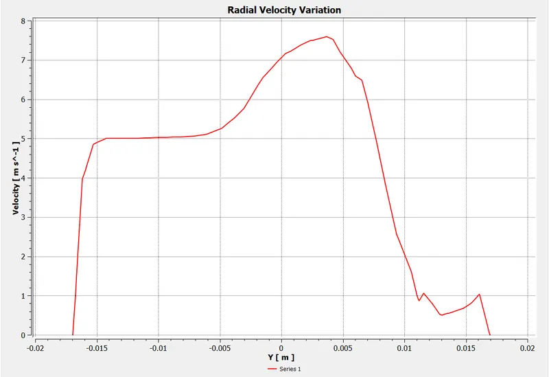
Fig. 15 (a)Temperature Variation along axis (b)Velocity Variation along axis (c)Temperature Variation along Radius (just after Tee-junction) (d)Velocity Variation along Radius (just after Tee-junction)
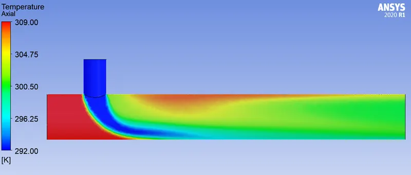
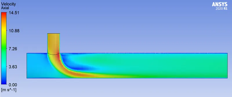
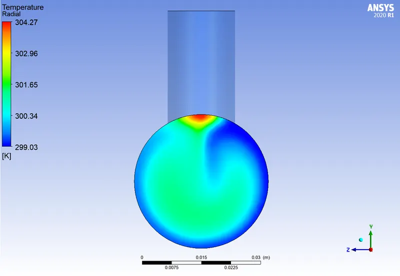
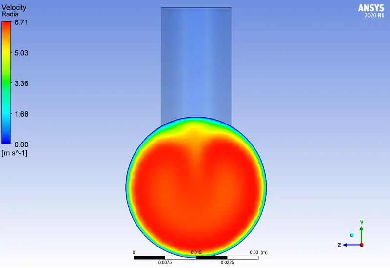
Momentum Ratio:4
(a) (b)
(c) (d)
Fig. 16 (a) Axial Plane Temperature Variation (b) Axial Plane Velocity Variation (c) Radial Plane Temperature Variation (outlet) (d) Radial Plane Velocity Variation (outlet)
(a) (b)
(c) (d)
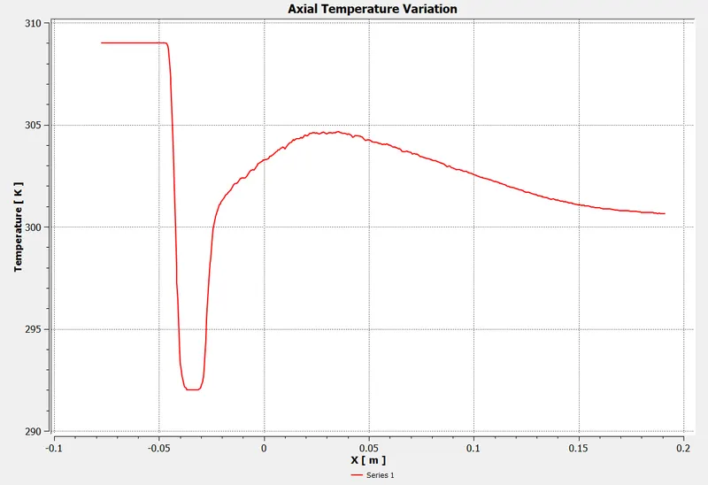
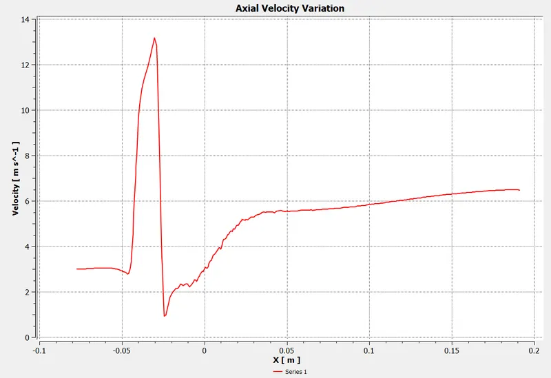
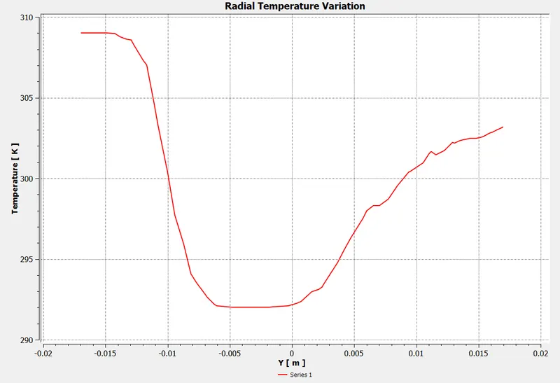
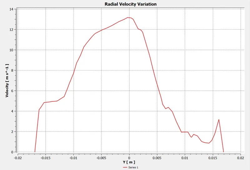
Fig. 17 (a)Temperature Variation along axis (b)Velocity Variation along axis (c)Temperature Variation along Radius (just after Tee-junction) (d)Velocity Variation along Radius (just after Tee-junction)
FINAL TABULATED COMPARISON OF EACH TEST CASE:
The diameter of the hot inlet and outlet pipe is 0.02m, and that of cold inlet pipe is 0.01m.
Table 3 Comparison of all test cases with theoretical data
| TEST CASES | MR=2, SHORT | MR=4, SHORT | MR=2, LONG | MR=4, LONG | THEORETICAL MR=2 | THEORETICAL MR=4 |
| Number of Tetrahedral cells | 574194 | 574194 | 761990 | 761990 | - | - |
| Number of Iterations | 125 | 191 | 120 | 174 | - | - |
| Standard Deviation for Velocity | 0.762 m/s | 0.7144 m/s | 0.901 m/s | 0.988 m/s | - | - |
| Area Weighted Average Velocity | 4.514 m/s | 6.055 m/s | 4.508 m/s | 6.034 m/s | 4.500 m/s | 6.000 m/s |
| Standard Deviation for Temperature | 1.921 K | 1.334 K | 1.220 K | 0.766 K | - | - |
| Area Weighted Average Temperature | 303.407 K | 300.550 K | 303.410 K | 300.479 K | 303.333 K | 300.500 K |
CONCLUSION:
Convergence is observed in the `k-epsilon` turbulence model.
Finer mesh cell size gives better details of the flow near the junction.
The outlet flow variables show less error for Long Geometry case, as more length is travelled by the flow to stabilize and reach steady state.
Both temperature and velocity line plots at the Tee-junction show mixing phenomenon and fluctuation in the respective properties.
The bounded nature of the flow is satisfied as the velocity and temperature are always within the higher and lower value range (No fluctuation or discontinuity).
The reason `k-omega` turbulence model does not show convergence in the Console is because the tolerance level is set to `1e^(-6)`. The Residual values were stable, but did not minimize to the stated tolerance level.
A higher momentum ratio resulted in lowering of the final outlet temperature and increase in the outlet velocity.