CFD Simulation of Cyclone Separator using Discrete Phase Modelling in ANSYS Fluent

CFD SIMULATION OF CYCLONE SEPARATOR USING DISCRETE PHASE MODELLING

AIM: To perform analysis on cyclone separator and calculate the separation efficiency and pressure drop.

OBJECTIVE:

1. To write a few words about any four empirical models used to calculate the cyclone separator efficiency.
2. To perform an analysis on a given cyclone separator model by varying the particle diameter from 1 μm to 5 μm and calculate the separation efficiency in each case. Discuss the results. [Use both the velocity's as 3m/sec.]
3. To perform an analysis on a given cyclone separator model by varying the particle velocity from 1 m/sec to 5 m/sec and calculate the separation efficiency and pressure drop in each case. Discuss the results. [Use particle diameter size as 5 μm for all cases & keep flow velocity same as particle velocity]

INTRODUCTION:

Cyclone separators are separation devices that use the principle of inertia to remove particulate matter from flue gases. Cyclone separator is one of many air pollution control devices known as precleaners since they generally remove larger pieces of particulate matter. This prevents finer filtration methods from having to deal with large, more abrasive particles later on. In addition, several cyclone separators can operate in parallel, and this system is known as a multicyclone.Cyclones can vary drastically in their size. The size of the cyclone depends largely on how much flue gas must be filtered, thus larger operations tend to need larger cyclones.

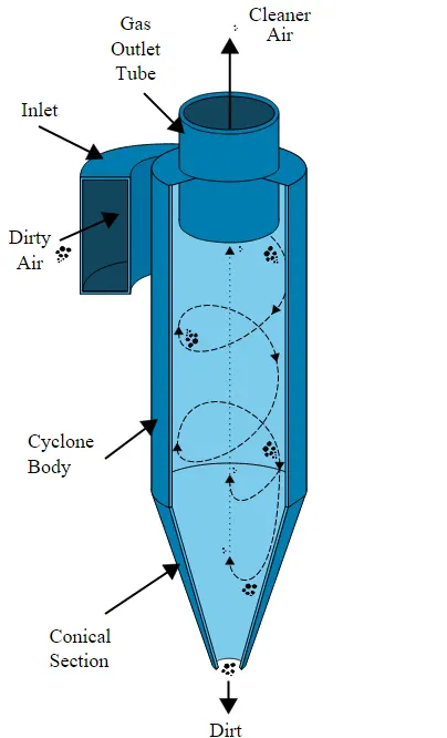
Fig. 1 Cyclone Separator Schematic

Cyclone separators work much like a centrifuge, but with a continuous feed of dirty air. In a cyclone separator, dirty flue gas is fed into a chamber. The inside of the chamber creates a spiral vortex, similar to a tornado. This spiral formation and the separation is shown in Fig. 2. The lighter components of this gas have less inertia, so it is easier for them to be influenced by the vortex and travel up it. Contrarily, larger components of particulate matter have more inertia and are not as easily influenced by the vortex.

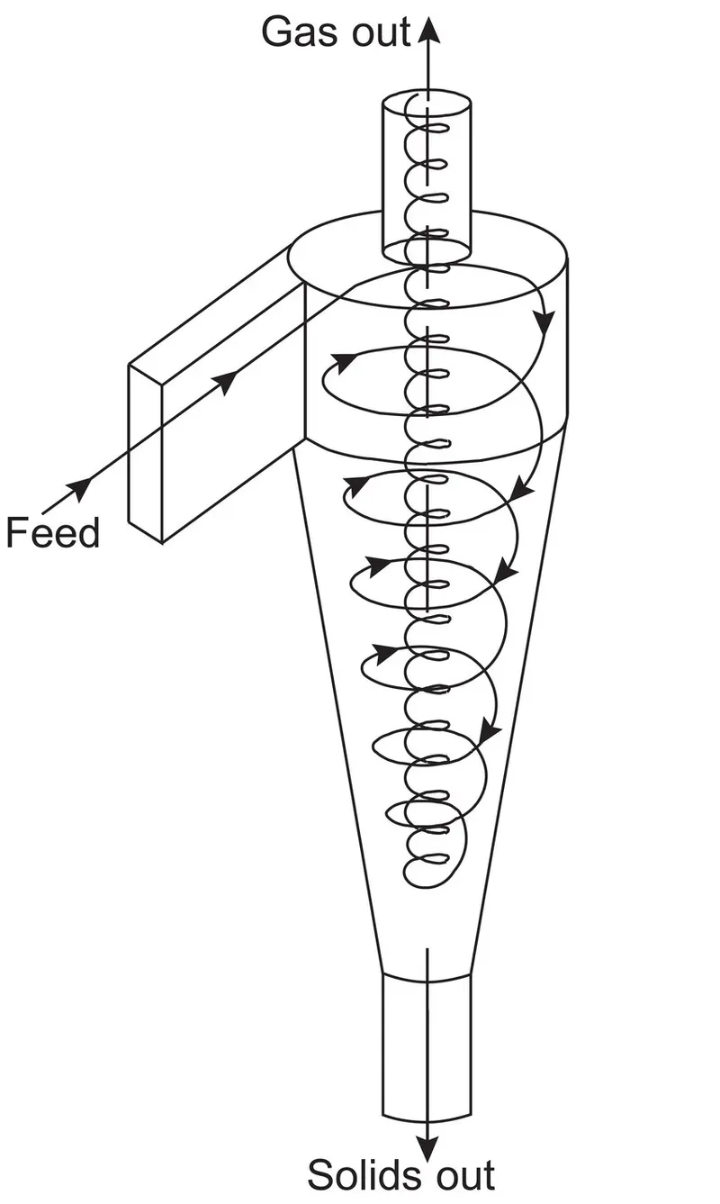
Fig. 2 Working pathway in a cyclone separator

Empirical Models for Cyclone Separator Efficiency:

1. Iozia and Leith Model:

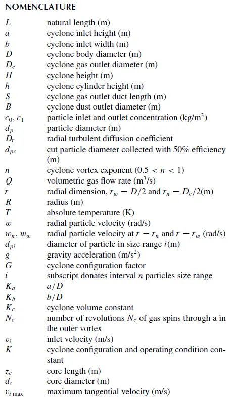
Iozia and Leith logistic model is a modified version of Barth Model, which is developed based on force balance. The model assumes that a particle carried by the vortex endures the influence of two forces: a centrifugal force, `Z` and a flow resistance, `W`. The collection efficiency `eta_i` of particle diameter `d_(text(pi))` can be calculated from
`eta_i=1/(1+(d_(pc)/d_(text(pi)))^beta)`
`beta` is an expression for slope parameter derived based on the statistical analysis of experimental data of a cyclone with D = 0.25 m given as
`beta=0.62-0.87ln(d_(pc)/100)+5.21ln((ab)/D^2)+1.05[ln((ab)/D^2)]^2`

and `d_(pc)` is the 50% cut size.

2. Li and Wang Model:

The Li and Wang model includes particle bounce or re-entrainment and turbulent diffusion at the cyclone wall. A two-dimensional analytical expression of particle distribution in the cyclone is obtained. Li and Wang model was developed based on the following assumptions:
• The radial particle velocity and the radial concentration profile are not constant for uncollected particles within the cyclone.
• Boundary conditions with the consideration of turbulent diffusion coefficient and particle bounce re-entrainment on the cyclone wall are:

`c=c_0` at `theta=0`

`D_r(delc)/(delr)=(1-alpha)wc` at `r=D/2`

• The tangential velocity is related to the radius of cyclone by: `uR^n = text(constant)`.

The resultant expression of the collection efficiency for particle of any size is given as

`eta_i=1-exp{-lamdatheta_1}`

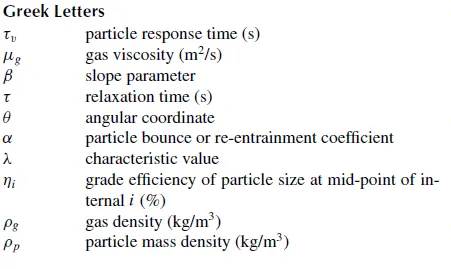
where `theta_1=2pi(S+L)/a` and `lamda=((1-alpha)Kw_w)/(D_rr_w^n)`

3. Koch and Licht Model:

Koch and Licht collection theory recognized the inherently turbulent nature of cyclones and the distribution of gas residence times within the cyclone. Koch and Licht described particle motion in the entry and collection regions with the additional following assumptions:
• The tangential velocity of a particle is equal to the tangential velocity of the gas flow, i.e. there is no slip in the tangential direction between the particle and the gas.
• The tangential velocity is related to the radius of cyclone by: `uR^n = text(constant)`.

A force balance and an equation on the particles collection yields the grade efficiency:

`eta_i=1-exp{-2[(Gtau_iQ)/D^3(n+1)]^(0.5/(n+1))}`

where `G=(8K_c)/(K_a^2K_b^2)` `n=1-{1-((12D)^0.14)/(2.5)}{(T+460)/530}^0.3` `tau_i=rho_pd_(text(pi))^2/(18mu)`

4. Lapple Model:

Lapple model was developed based on force balance without considering the flow resistance. Lapple assumed that a particle entering the cyclone is evenly distributed across the inlet opening. The particle that travels from inlet half width to the wall in the cyclone is collected with 50% efficiency. The semi empirical relationship developed by Lapple to calculate a 50% cut diameter, `d_(pc)`, is

`d_(pc)=[(9mub)/(2piN_ev_i(rho_p-rho_g))]^(1/2)`

where `N_e=1/a[h+(H-h)/2]`

and `eta_i=1/(1+(d_(pc)/d_(text(pi)))^2)`

Through literature, it was found out that the Li and Wang Model and CFD Code cyclone efficiency. The cyclone efficiency using the CFD Code is calculated by:

`eta=(text(Number of particles trapped))/(text(Number of particles injected - incomplete))`

The phase modelling involves two phases:

Continuous Phase, is the main fluid continuum phase.

Discrete Phase includes a large number of particles in the flowing Continuous Phase.

The Discrete Phase Modelling (DPM) in ANSYS Fluent predicts the trajectory of the discrete particles by integrating the force balance on the particles. DPM can be carried out using two methods, Coupled Flow in which the Discrete Phase has an interaction with the Continuous Phase and Uncoupled Flow where it does not. For the current analysis, since the particle size is very small the interaction with both the phases is neglected.

SOLVING AND MODELLING APPROACH:

The following flow chart is followed for the Solving Approach:

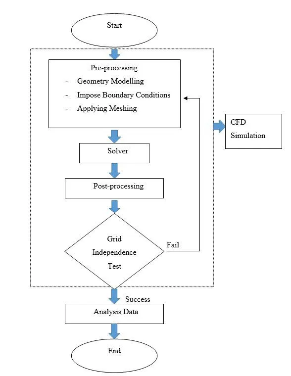
Fig. 4 Solving Approach Flow Chart

ANSYS involves selection of Fluent solver, input and verification of Geometry, Meshing, Setup, Solutions and Results. The Geometry is input in ANSYS Space Claim. The mesh sizing and face naming is done while Meshing. The Setup section involves Mesh Checking, Turbulence Model selection, Solver type, velocity formulation and time (steady or transient state), Output report files, Material selection, Initial and Boundary conditions. The Results section is used for the visualiztion of the output in a GUI.

PRE-PROCESSING AND SOLVER SETTINGS:

GEOMETRY:

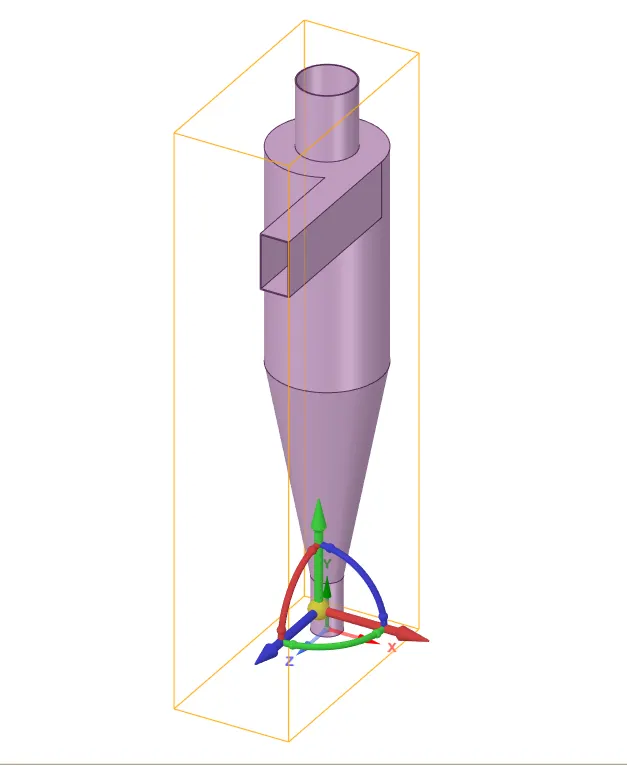
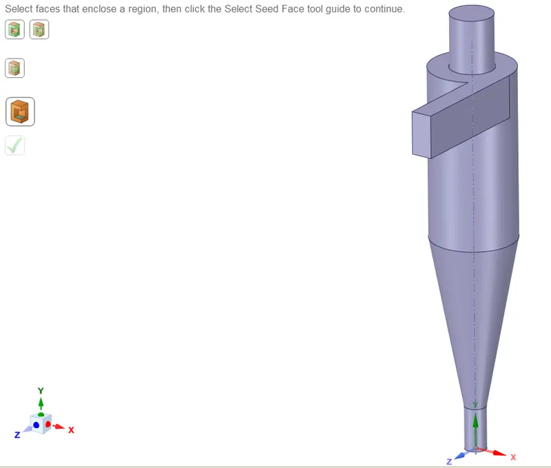
(a) (b)

Fig. 1 (a)CAD Geometry for Cyclone Separator ,(b) Extracted enclosure geometry

The above geometry is imported into Spaceclaim. Volume extract feature is used to create a volume where the fluid flows. The Cyclone Separator geometry is Suppressed for Physics to only consider the enclosure for fluid interactions.

MESHING:

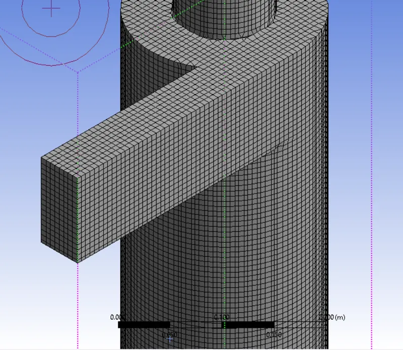
Fig. 2 Meshing for the Geometry

A baseline mesh was created with element size of 14.2 mm. The respective faces were named Inlet, Outlet-Top and Outlet-Bottom. The wall condition is automatically taken by Fluent for the un-named faces. Method option in Insert was used to create a Cartersian Meshing Method. The Element Size for the Method input was set to `5e^(-3)`.

SETUP:

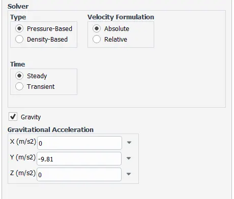
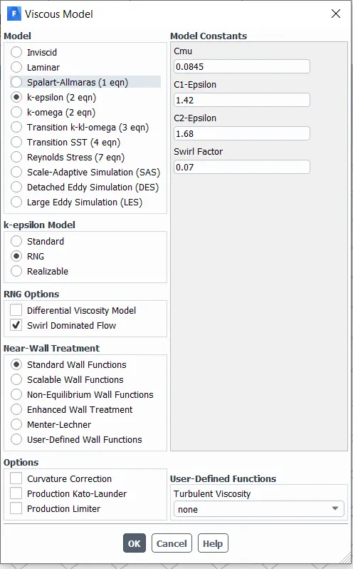
Since the problelm statement is considered for a low Mach number, a Pressure Based Solver is considered for the simulation. The `k-epsilon` RNG Turbulence model was used for the respective test case calculations. In the model Swirl Dominated Flow is activated. This improves the accuracy for a swirling flow.

(a) (b)

Fig. 3 (a)Setup- Solver, (b) Setup- Viscous Model

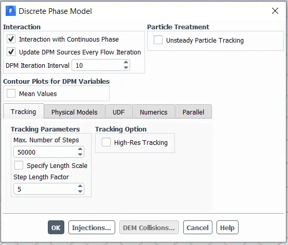
A Steady State simulation is run. In the Physics section, Discrete Phase Modelling option is enabled. The Interact with continuous phase and Update DPM Sources option are enabled for smooth computation.

(a) (b)

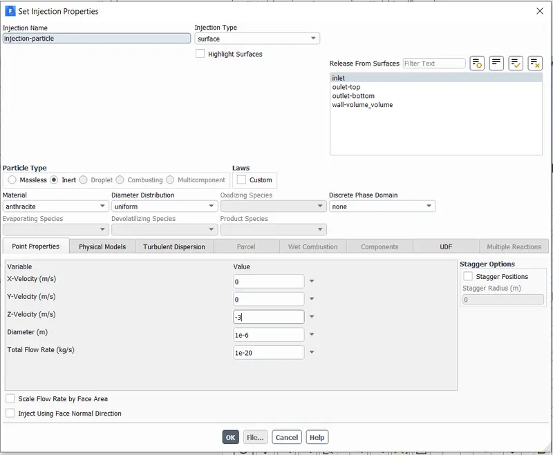
Fig. 4 (a) Discrete Phase Modelling Setup, (b) DPM- Injection Input Setup

The Tracking settings are left as default. The Injections Section is opened, and a new Injection is created, wherein the Injection Type-Surface is input. This enables the whole inlet face to inject the particles. The inlet phase is selected on the Surface panel. Anthracite material is chosen and the diameter and velocity is input. In Boundary Conditions input to the faces, the Inelt phase is given the same velocity as the particle, and DPM Phase BC as Reflect. This is to reflect any particle falling onto the phasse. The walls are also given the Reflect DPM Phase BC, the Outlet-Bottom is given a Trap BC and Oulet-Top is given the Escape BC. Each boundary condition is named by the characterstic of the DPM particles behaviour intended on interaction with the particular phase.

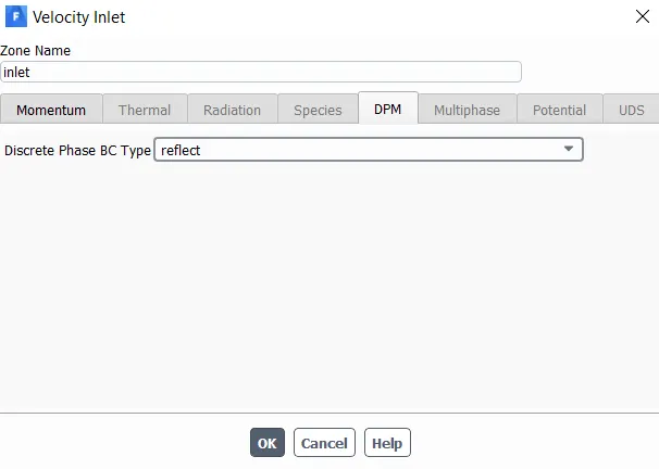
Fig. 5 Boundary Condition Setup example for Inlet Phase

The Solution Methods for the Setup is set to Second Order Upwind for Turbulent k, dissipation and momentum computations. The Standard Initialization is used wherein the user inputs the initial velocity and face from where computation will start.

The simulation is run for 1000 iterations and the

The Fluent Particle Track File was Written in Fluent and the Results were tracked in CFD Post.

RESULTS:

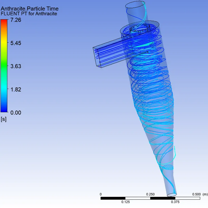
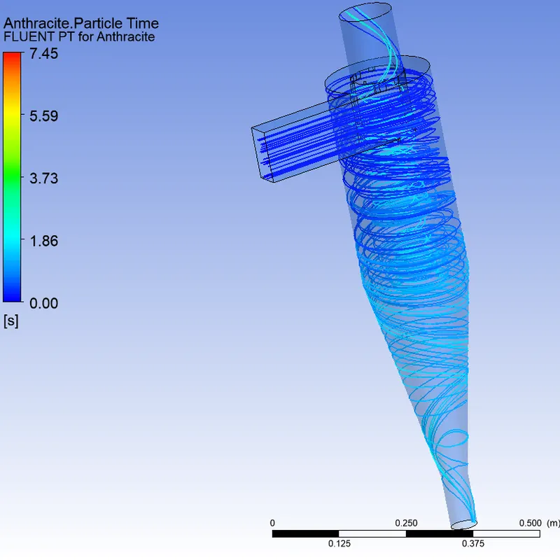
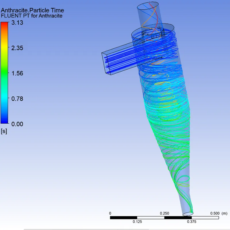
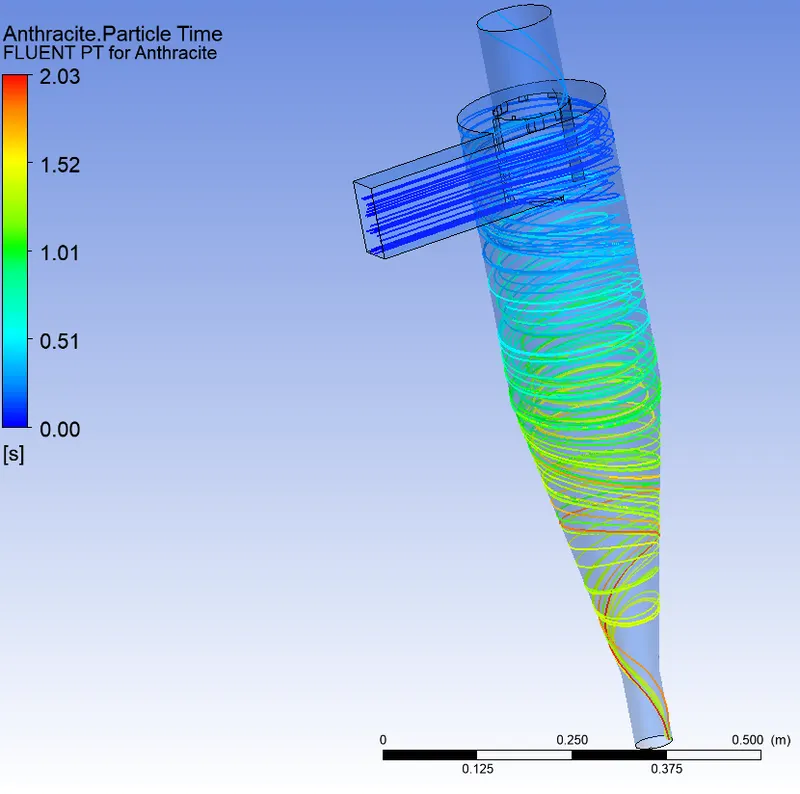
TEST 1: Variation of Particle Size

Particle Diameter: D

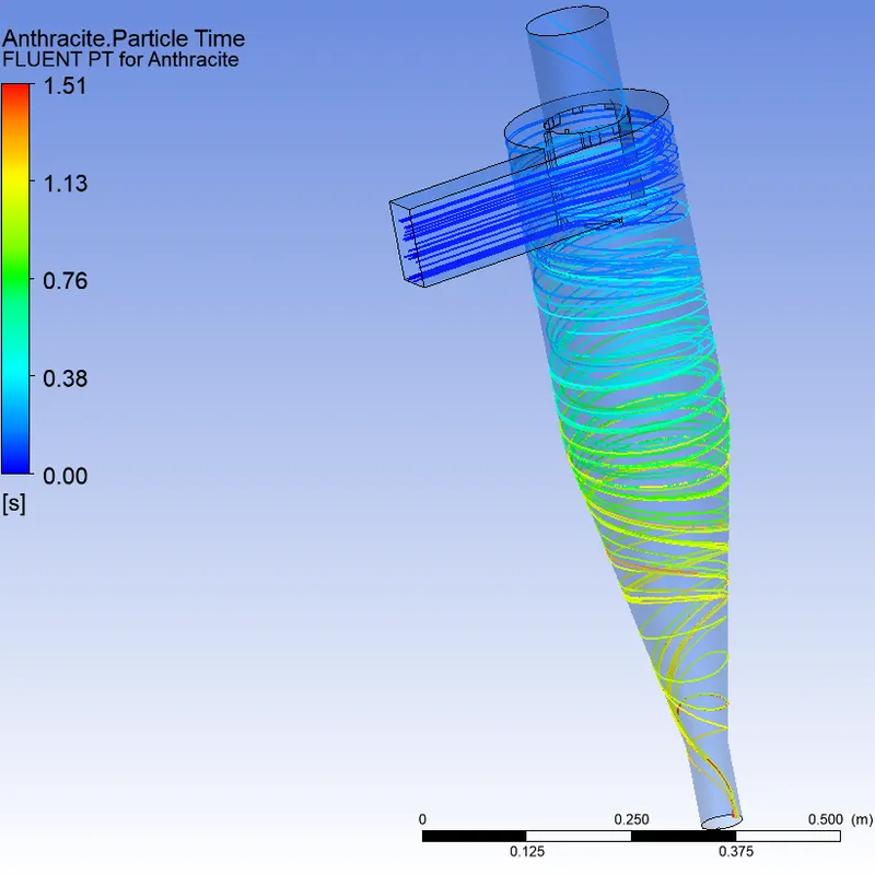
Velocity=3 m/s	Particle Pressure Variation	Particle Time to escape/trap
D= `1 mum`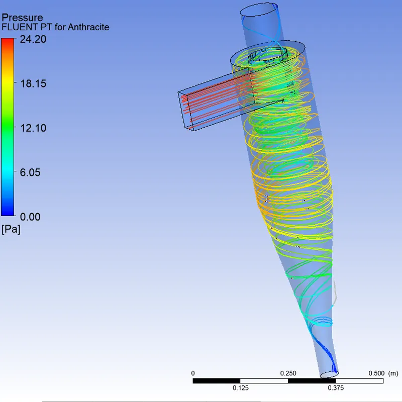
D= `2 mum`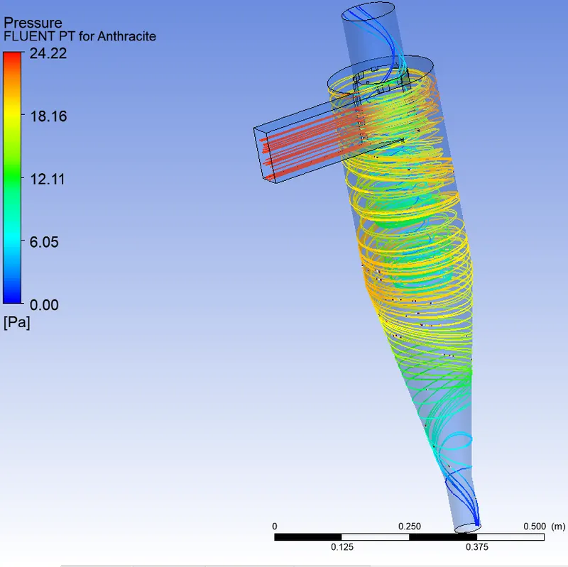
D= `3 mum`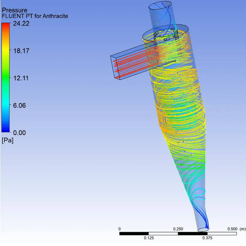
D= `4 mum`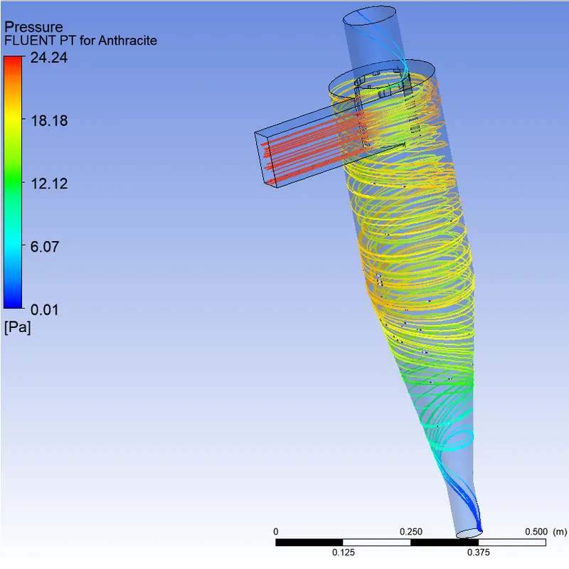
D= `5 mum`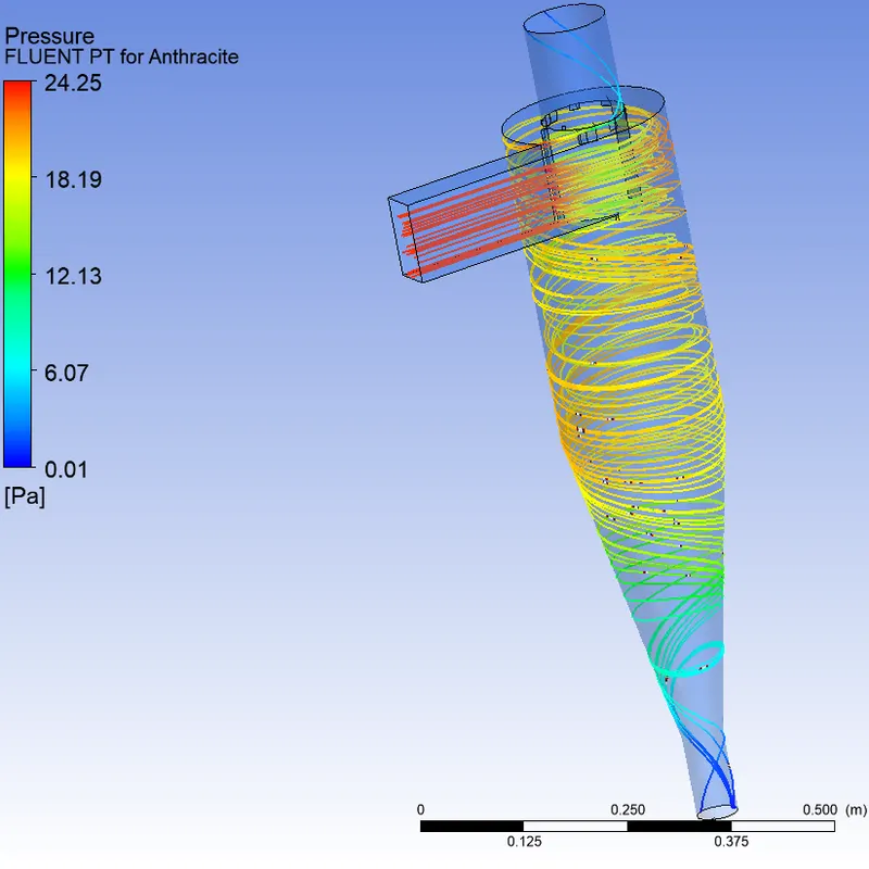

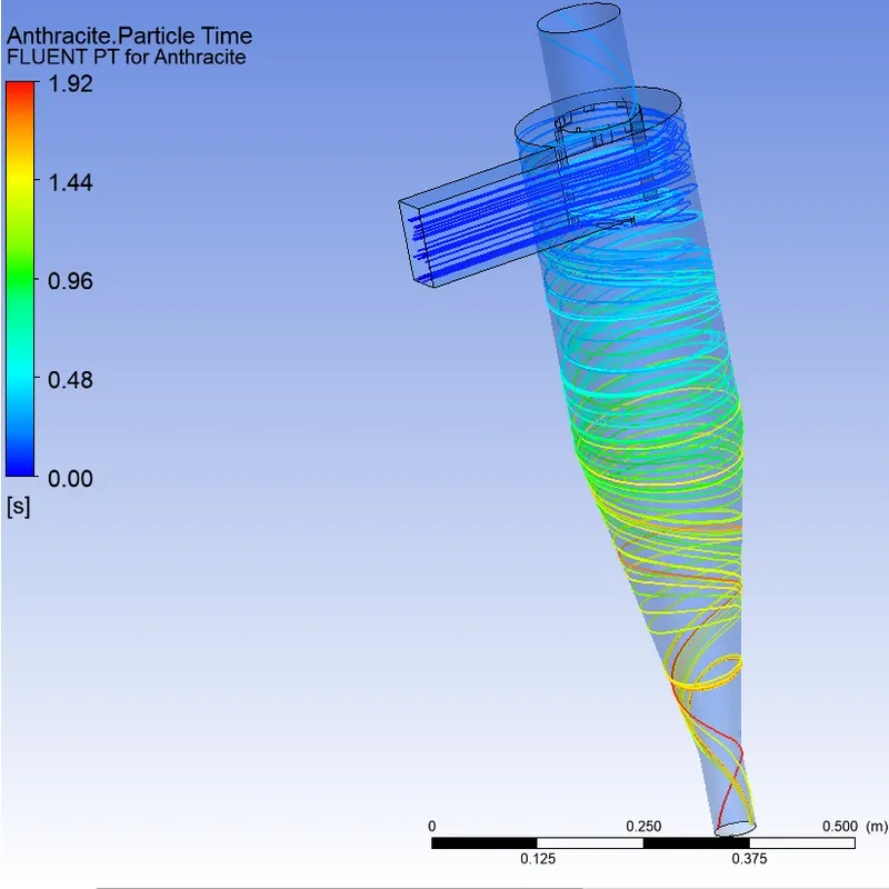Tabulated Pressure and DPM Tracking values:

v=3 m/s	Total Pressure at Inlet (Pa)	Total Pressure at Outlet Top (Pa)	Pressure Drop (Pa)	Number of particles Tracked	Number of particles Escaped	Number of particles Trapped	Number of particles Incomplete	Separation Efficiency (%)
`D=1mum`	29.02	4.23	24.79	136	31	84	21	73.04
`D=2mum`	29.02	4.23	24.79	136	25	91	20	78.45
`D=3mum`	29.02	4.23	24.79	136	31	100	5	76.33
`D=4mum`	29.02	4.23	24.79	136	18	118	0	86.76
`D=5mum`	29.02	4.23	24.79	136	19	117	0	86.03

TEST 2: Variation of Particle Speed

Flow and Particle Velocity: V

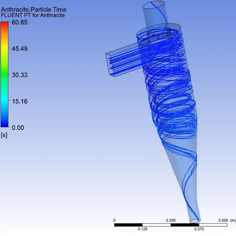
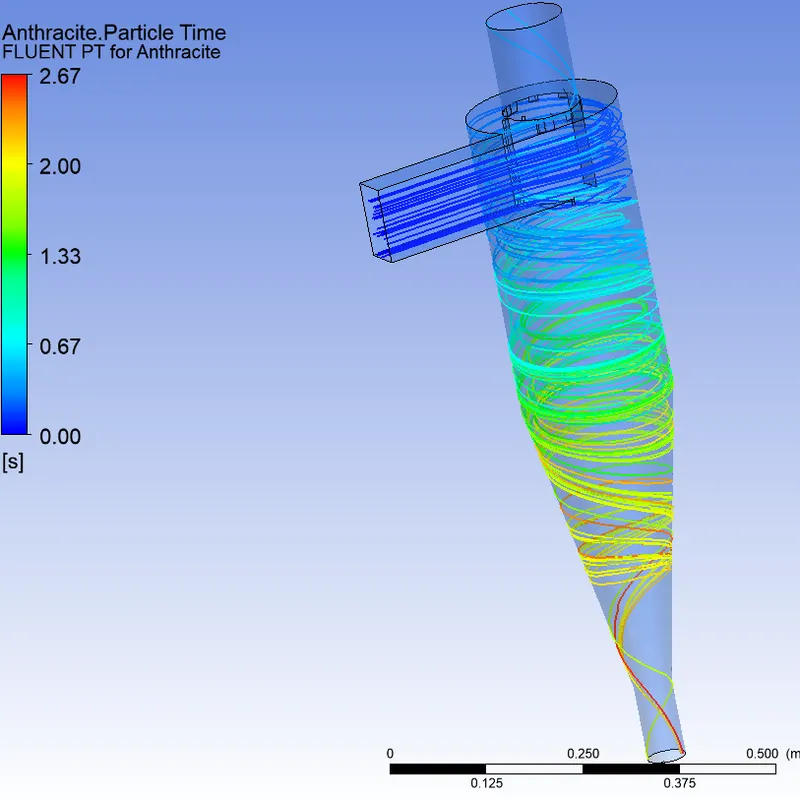
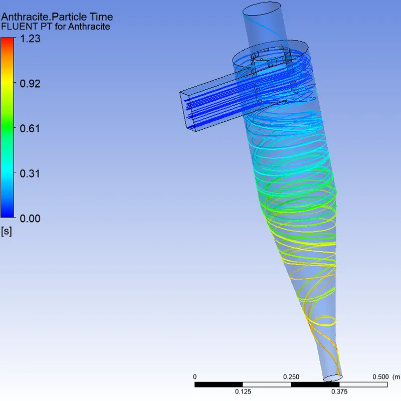
Diameter=`5mum`	Particle Pressure Variation	Particle Time to escape/trap
V= 1 m/s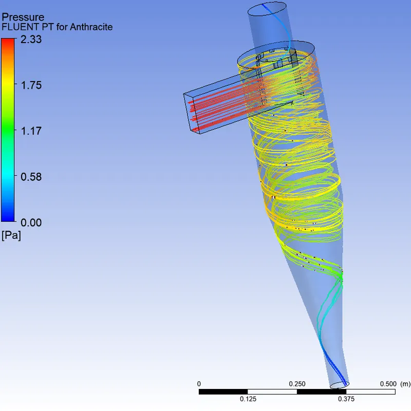
V= 2 m/s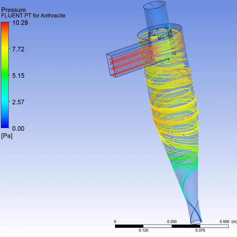
V= 3 m/s
V= 4 m/s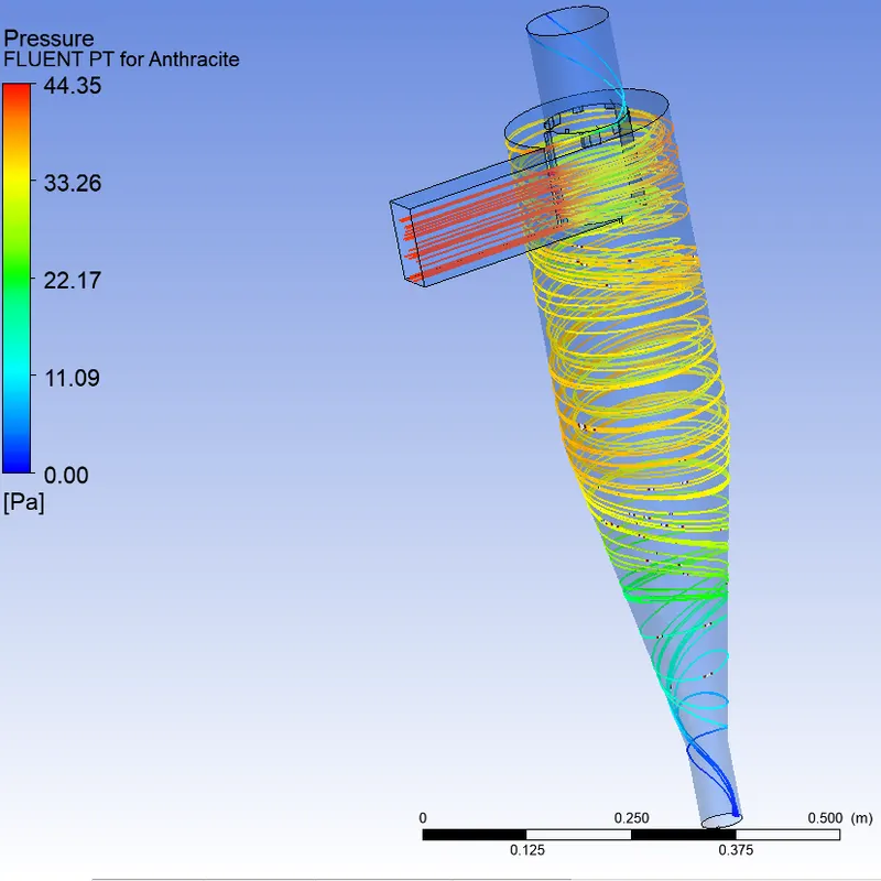
V= 5 m/s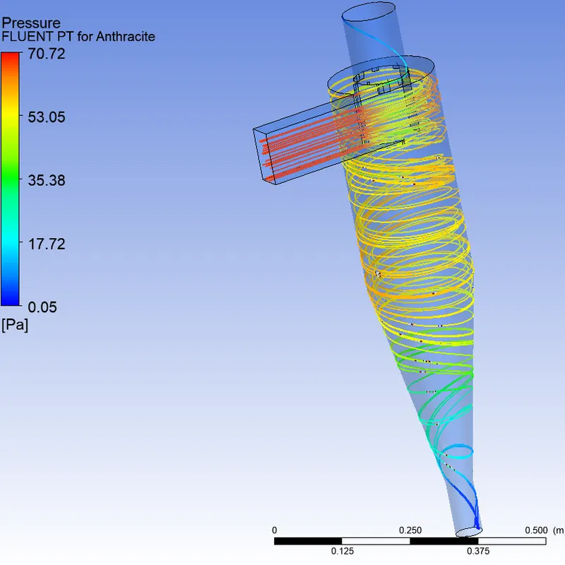

Tabulated Pressure and DPM Tracking values:

D=`5mum`	Total Pressure at Inlet (Pa)	Total Pressure at Outlet Top (Pa)	Pressure Drop (Pa)	Number of particles Tracked	Number of particles Escaped	Number of particles Trapped	Number of particles Incomplete	Separation Efficiency (%)
V=1 m/s	2.91	0.40	2.50	136	30	84	22	73.68
V=2 m/s	12.47	1.79	10.68	136	18	118	0	86.76
V=3 m/s	29.02	4.23	24.79	136	19	117	0	86.03
V=4 m/s	52.70	7.75	44.95	136	17	119	0	87.50
V=5 m/s	83.62	12.36	71.26	136	19	117	0	85.03

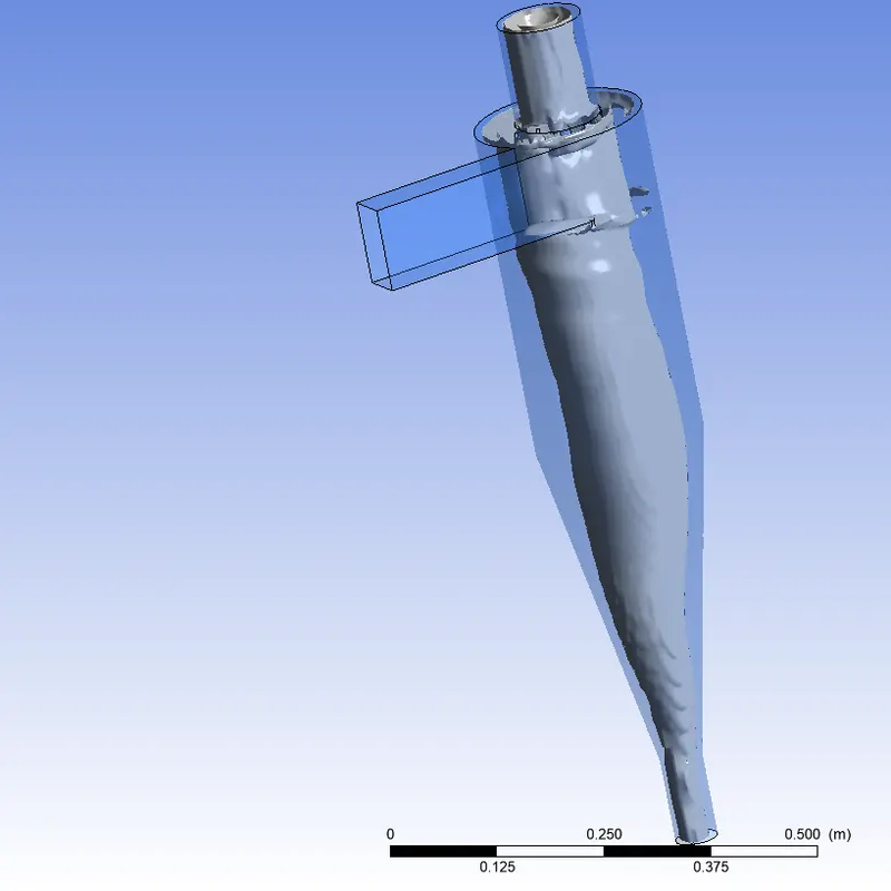
Fig. 6 Vortex Core Region generated in every experiment

Animation for the Particle Tracking History recorded [Test 1: Case 1]:

CONCLUSION:

The Vortex Core Region results are similar for each test case. Therefore, it can be concluded that the particle diameter and velocity of injection do not play a role in the Vortex formed.

As the diameter of the particles is increased (TEST 1), no change in pressure drop is observed and an increase in separation efficiency is observed.

As the velocity of injection and flow is increased (TEST 2), the minimal difference in separation is observed after 2 m/s simulation. There is a drastic change in pressure drop observed, as the particle and flow velocity affect the total pressure on each face.

The particle tracking time reduces as the diameter of the particle increases and the velocity of the particle increase.