Conjugate Heat Transfer Simulation in an Exhaust Port using ANSYS Fluent

CONJUGATE HEAT TRANSFER SIMULATION OF EXHAUST PORT

AIM:

To run an ANSYS Fluent simulation on an IC Engine Exhaust port and observe the Conjugate Heat transfer results.

Maintain the y+ value according to the turbulence model and justify the results.

Calculate the wall/surface heat transfer coefficient on the internal solid surface & show the velocity & temperature contours in appropriate areas.

INTRODUCTION:

Q:Give a brief description of why and where a Conjugate Heat Transfer analysis is used.

A:

Conjugate heat transfer corresponds with the combination of heat transfer in solids and heat transfer in fluids. In solids, conduction often dominates whereas in fluids, convection usually dominates. Conjugate heat transfer is observed in many situations. For example, heat sinks are optimized to combine heat transfer by conduction in the heat sink with the convection in the surrounding fluid.

Effective Heat Transfer

Efficiently combining heat transfer in fluids and solids is the key to designing effective coolers, heaters, or heat exchangers.

The fluid usually plays the role of energy carrier on large distances. Forced convection is the most common way to achieve high heat transfer rate. In some applications, the performances are further improved by combining convection with phase change (for example liquid water to vapor phase change).

Even so, solids are also needed, in particular to separate fluids in a heat exchanger so that fluids exchange energy without being mixed.Heat sinks are usually made of metal with high thermal conductivity (e.g. copper or aluminum). They dissipate heat by increasing the exchange area between the solid part and the surrounding fluid.

Energy Savings

Heat transfer in fluids and solids can also be combined to minimize heat losses in various devices. Because most gases (especially at low pressure) have small thermal conductivities, they can be used as thermal insulators… provided they are not in motion. In many situations, gas is preferred to other material due to its low weight. In any case, it is important to limit the heat transfer by convection, in particular by reducing the natural convection effects. Judicious positioning of walls and use of small cavities helps to control the natural convection. Applied at the micro scale, the principle leads to the insulation foam concept where tiny cavities of air (bubbles) are trapped in the foam material (e.g. polyurethane), which combines high insulation performances with light weight.

Q:How would you verify if the Heat Transfer Coefficient predictions from the simulations are right? On what factors does the accuracy of the prediction depend on?

A:

Convective Heat Transfer coefficient depends on factors: Flow velocity, Turbulence model, viscocity and geometry of the body or pipe. The Newton's Law of Cooling states that:

`Q=hA(T_1-T_2)`

where `Q` is the wall heat flux, and `T_1` and `T_2` are the respective temperatures of two bodies. This appliedd to convection transforms to give HTC:

`h=q/(T_(wall)-T_(ref))`

where `q` is the wall heat flux per unit area, `T_(wall` is the wall temperature and `T_(ref)` is the fluid temperature. Calculation of this reference fluid temperature is the key aspect of HTC calculation. The fluid temperature varies near the wall due to thermal boundary layer as shown below:

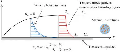
Fig. 1 Velocity and Thermal Boundary Layer on a flat plate

For internal flow the, the reference temperature is the mass flow average temperature

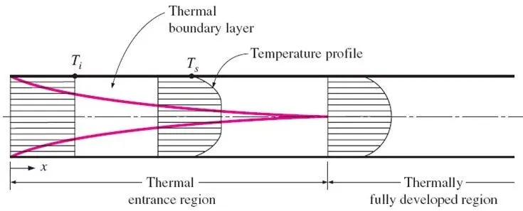
Fig. 2 Thermal Boundary Layer- Internal Flow

The Mass flow average is given by:

`T_(ref)=1/(dotm)int_ArhoUTdA`

CFD codes use two different methods to define `T_(ref)`:

1. Temperature at the centroid of the cell nearest to the wall

2. User Manual Input of `T_(ref)`

Nearest Cell Centroid:

This reference temperature is defined based on whether the CFD code is using Wall Functions:

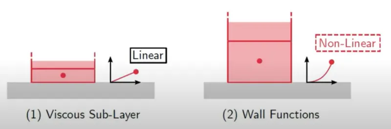
Fig. 3 Viscous Sub Layer and Wall Function reference temperature computation

Assuming the temperature function is given by a function: `T^+=f(y^+)`, where `T^+` is defined by:

`T^+=((T_(wall)-T_(cell))rhoC_pC_mu^(1/4)k^(1/2))/(q)`

Applying the definition to HTC:

`h=q/(T_(wall)-T_(cell))rightarrow h=(rhoC_pC_mu^(1/4)k^(1/2))/(T^+)`.

The respective function `f(y^+)` is used to calculate the `T^+` and then the HTC.

The problem with the Nearest Cell Wall modelling is that the `T_(ref)` is Mesh dependent. More refined the mesh, the centroid of the cell is more closer to the wall, which affects the `y^+` and hence the `T^+`. This can only be validated through experimental data.

A better approach to input the `T_(ref)` accurately would be through manual input. Inputting the correct temperature through Reference Values column in ANSYS Fluent.

Note: The Surface Heat Transfer plot should be plotted rather than the Wall Heat Transfer, as Fluent is equipped to using both Manual input and Nearest Cell Centroid method. The Manual input result is shown on using the Surface plot.

The Heat Transfer Coefficient is also calculated theoretically using the Nusselt Number and Prandtl Number:

`Nu=0.023.Re^(0.8)Pr^(0.4)`

`Nu=(hL)/k`

where `k` is the material's conductivity.

GOVERNING EQUATIONS AND THEORY:

`text(SST k-omega)` resolves the boundary layer in the viscous sub-layer. A `y^+~1` for closure is needed to take advantage of this resolution. If `y^+>20` the `k-omega` part of the SST model is not used and simply reduces to `k-epsi` model.

SOLVING AND MODELLING APPROACH:

The following flow chart is followed for the Solving Approach:

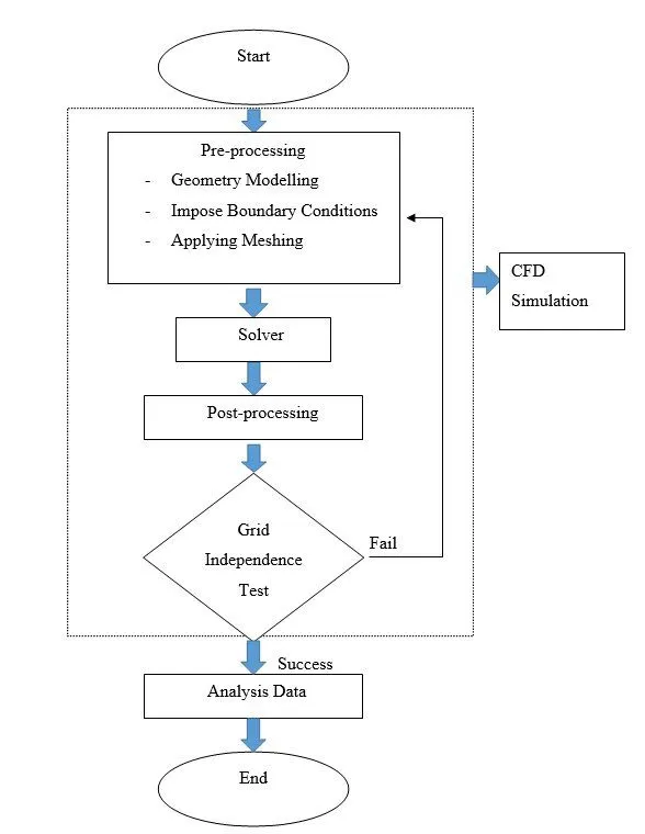
Fig. 4 Solving Approach Flow Chart

ANSYS involves selection of Fluent solver, input and verification of Geometry, Meshing, Setup, Solutions and Results. The Geometry is input in ANSYS Space Claim. The mesh sizing and face naming is done while Meshing. The Setup section involves Mesh Checking, Turbulence Model selection, Solver type, velocity formulation and time (steady or transient state), Output report files, Material selection, Initial and Boundary conditions. The Results section is used for the visualiztion of the output in a GUI.

PRE-PROCESSING AND SOLVER SETTINGS:

The input conditions involve inlet flow velocity of `u_0=25text( m/s)`.

GEOMETRY:

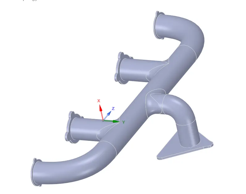
Fig. 5 CAD Geometry for Exhaust Port

The above geometry is imported into Spaceclaim. Volume extract feature is used to create a volume where the fluid flows. Share Topology and Share Prep options should be enabled for the flow information to commute between the two bodies. The Share topology option also ensures that a Conformal Mesh is created. Since this is a Conjugate Heat Transfer case, the tow bodies- Exhaust Port and Volume Extract (Fluid Volume) are moved to a new single component.

MESHING:

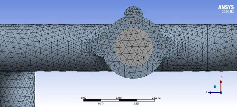
Fig. 6 Meshing for the Geometry

A baseline mesh was created for first case. And a refined mesh with inflation layer at the inlet and outlet boundaries for the second case. The respective faces were named Inlet, Outlet and Outer Wall convection (for outer casing). No wall conditions are imposed to the Fluid Volume casing as flow information needs to flow across the two bodies.

SETUP:

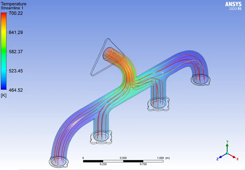
Since the problelm statement is considered for a low Mach number, a Pressure Based Solver is considered for the simulation. The `k-epsilon` Standard Turbulence model was used for the respective test case calculations. The Wall `y^+` value over the Fluid Volume is calculated to be maintained at `30. A Steady State simulation is run. The Boundary condition for the Inlet (Velocity=5 m/s and Temperature=700K), Outlet (Static Pressure= 1 atm) and Outer Wall Convection coefficient `20 W/(m^2K)`. Hybrid Initialization is used for t=0 and 300 iterations were run for each case. The temperature contours on the Outer Wall was plotted and the Wall Heat Transfer Coefficient in CFD Post.

RESULTS:

Case 1: Baseline Mesh

(a) (b)

(c) (d)

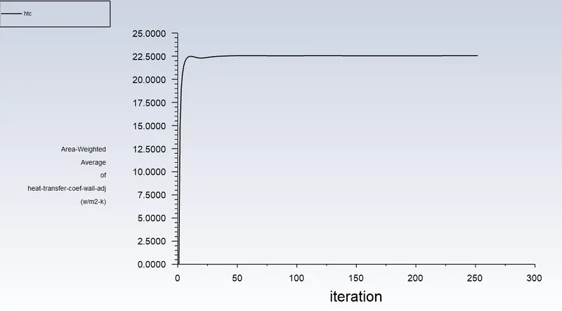
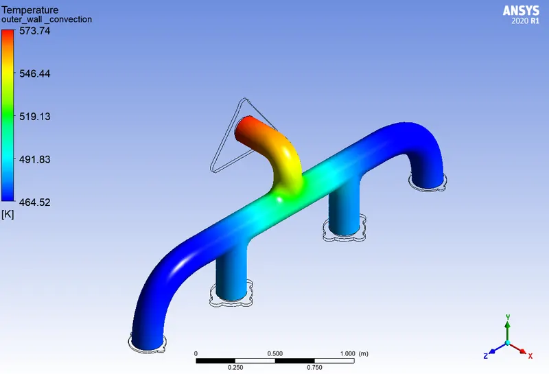
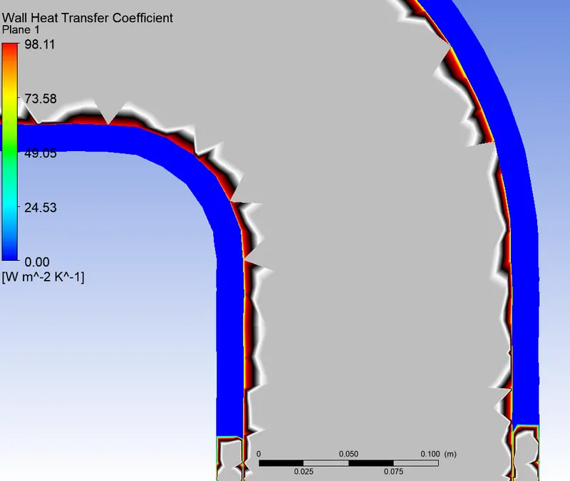
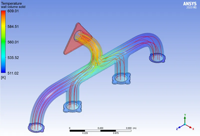
Fig. 7 (a) Heat Transfer Coefficient plot over number of iterations (b) Temperature variation over the Outer Wall (c) Velocity Streamlines with Temperature color plots (d) Wall Heat Transfer Coefficient contour on XY plane at outlet

Case 2: Refined Mesh

(a) (b)

(c) (d)

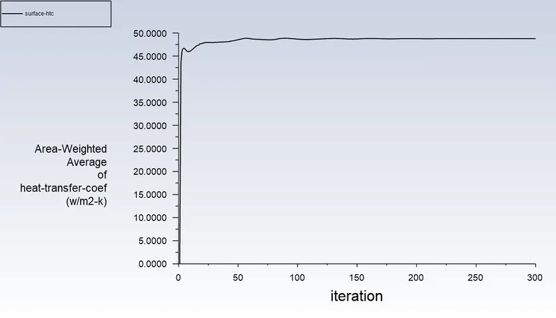
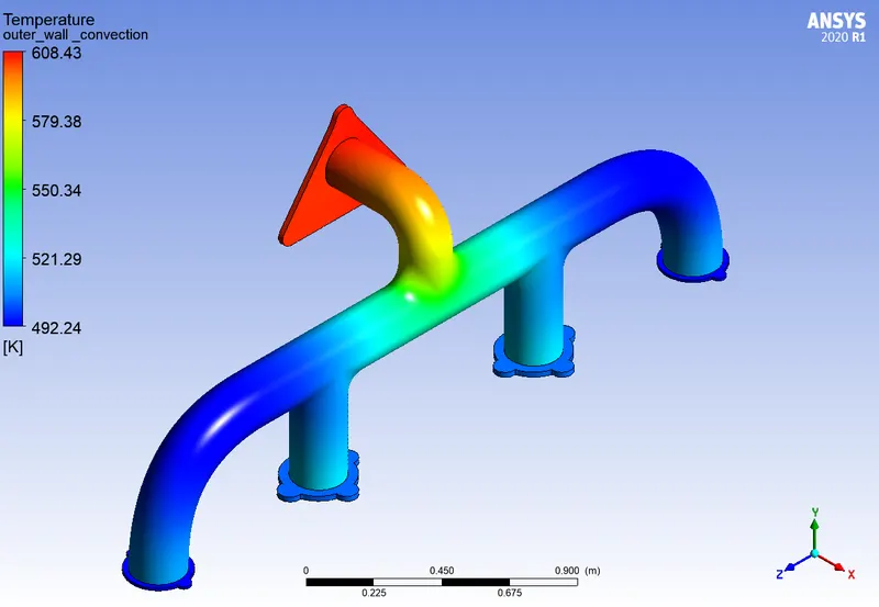
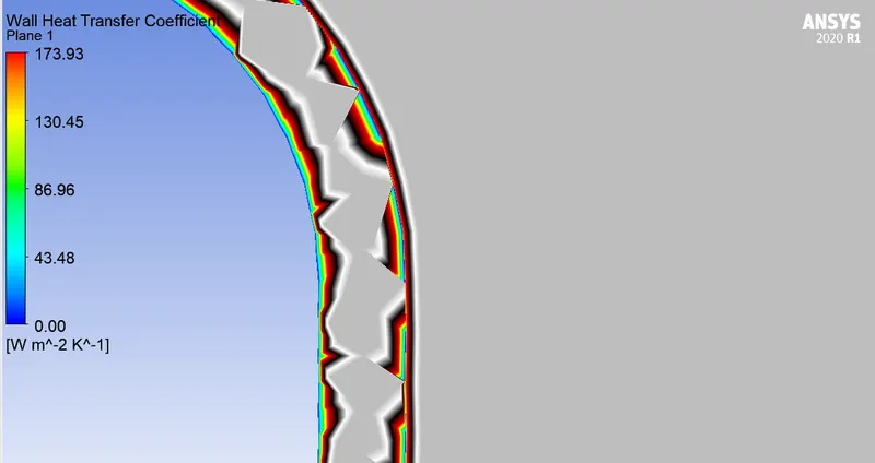
Fig. 8 (a) Heat Transfer Coefficient plot over number of iterations (b) Temperature variation over the Outer Wall (c) Velocity Streamlines with Temperature color plots (d) Wall Heat Transfer Coefficient contour on XY plane at outlet

The tabulated results and inputs of both test cases are stated below:

	Baseline Mesh	Refined Mesh
Element Size	0.15m	0.02m
Outer Wall Sizing	-	0.01m
Inflation Layer Total Thickness	-	20mm
Area Weighted Average Outlet Temperature	680.97K	678.16K
Area Weighted Average Heat Transfer Coefficient	`22.55W/(m^2K)`	`48.77 W/(m^2K)`
Maximum Wall Heat Transfer Coeffieicnt (CFD Post)	`98.11 W/(m^2K)`	`173.93W/(m^2K)`

The Area Weighted Average heat transfer coefficient is the calculation obtained in Fluent, where as the Maximum Heat Transfer Coefficient is obtained from CFD Post. `y^+=41.8` was considered for the `k-epsi` turbulence model. The Surface Heat Transfer Coefficient computation was used for the baseline mesh and the Wall Adjacent Heat Transfer Coefficient for the Refined Mesh. This is because the Nearest Node Centroid was not applicable for the Baseline Mesh, and a standard reference value was used for `T_(ref)`. The adjacent wall heat transfer function gives the right computation in the refined mesh case as the `y^+` and the turbulence model add to the `T^+` computation giving the right heat transfer coefficient value.

CONCLUSION:

The temperature profile was captured well by the Baseline mesh, and improved using the refined mesh.

Multiple heat transfer coefficient computations were tested to finalize the most applicable calculation.

CFD Post color mapping shows the Outer Wall temperature contour and how the heat transfer coefficient at the wall is affected by this.

The Refined Mesh computed convective heat transfer coefficient is closer to the extracted values from theory.