Conjugate Heat Transfer Simulation of Thermal Management System in a Graphic Card

CONJUGATE HEAT TRANSFER SIMULATION OF THERMAL MANAGEMENT SYSTEM IN A GRAPHIC CARD

AIM:

Perform a steady-state conjugate heat transfer analysis on a model of a graphics card. You can use appropriate materials of your choice for the simulation. Make sure to properly define the correct solid and fluid zones. Refer the video for further clarification and the model is provided below the video.

Run the simulation for best possible mesh with combination of coarse and refined mesh in different regions. Explain the reason for choosing the particular mesh settings.

Your Objectives:

1. Run the simulation by varying the velocity from 1m/sec to 5m/sec for at least 3 velocities and discuss the results.
2. Find out the maximum temperature and heat transfer coefficient attained by the processor.
3. Prove that the simulation has achieved convergence with appropriate images and plots.
4. Identify potential hotspots on the model.

INTRODUCTION:

The graphics processing cards typically consume more energy and demand more electrical power than central processing units. Accordingly, the graphics processing cards generate significant amounts of heat that can damage the components near the GPU or other devices in a host system, such as a computer or a game console. Manufacturers of graphics processing cards design heat dissipation systems for each individual GPU for each card model. The heat dissipation systems often include a fan and heat sink that are vertically stacked and positioned directly on top of the GPU. Every time a new graphics processing card is designed, a new heat dissipation system is designed. Since each heat dissipation system is associated with a single GPU and graphics processing card configuration, manufacturers must maintain a complex inventory of heat sink, fan, and other heat dissipation parts. This leads to higher costs of production as well as an increase in time-to-market for new designs.

GOVERNING EQUATIONS AND THEORY:

The thermal management system includes a mounting bracket that is configured to attach to each of the differently configured graphics processing cards. The mounting bracket has an opening that overlies the heat zone of the graphics processing card, which includes at least the graphics processing unit (GPU) or chip. The bracket is configured to be in thermal contact with the GPU and other heat generating components on the graphics processing card.

An arrangement of the components on each graphics processing card can vary depending on different design specifications, such as different memory requirements for different GPUs. Since the GPU is memory intensive, the memory is positioned within close proximity to the GPU in order to minimize the distance electrical signals must travel. The heat zone corresponds to an area of each graphics processing card where the GPU and the memory are positioned.

The thermal management system includes a heat sink that is configured to couple to the mounting bracket to be in thermal contact with the heat zone through the opening in the mounting bracket. The heat sink overlies at least a portion of the GPU that is positioned within the opening. The thermal management system also includes a fan that is configured to couple to the mounting bracket adjacent the heat sink. The fan incorporates an active heat transfer with the passive heat transfer of the heat sink.

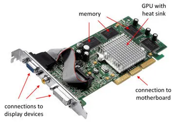
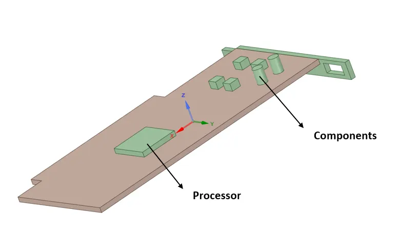
Fig. 1 Graphic Card components overview

SOLVING AND MODELLING APPROACH:

The following flow chart is followed for the Solving Approach:

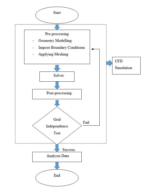
Fig. 4 Solving Approach Flow Chart

ANSYS involves selection of Fluent solver, input and verification of Geometry, Meshing, Setup, Solutions and Results. The Geometry is input in ANSYS Space Claim. The mesh sizing and face naming is done while Meshing. The Setup section involves Mesh Checking, Turbulence Model selection, Solver type, velocity formulation and time (steady or transient state), Output report files, Material selection, Initial and Boundary conditions. The Results section is used for the visualiztion of the output in a GUI.

PRE-PROCESSING AND SOLVER SETTINGS:

Initially the mesh dependency test is run for baseline and refined mesh at 3m/s inlet velocity. And then the velocity is varied (1m/s, 3m/s and 5m/s) to observe the heat dissipation.

GEOMETRY:

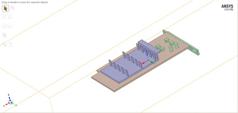
Fig. 1 CAD Geometry for Graphic Card

The above geometry is imported into Spaceclaim. An Enclosure is built around the body where the fluid will be flowing.. Share Topology and Share Prep options should be enabled for the flow information to commute between the two bodies. The Share topology option also ensures that a Conformal Mesh is created. Since this is a Conjugate Heat Transfer case, the two bodies- Graphic Card and Enclosure (Fluid Volume) are moved to a new single component.

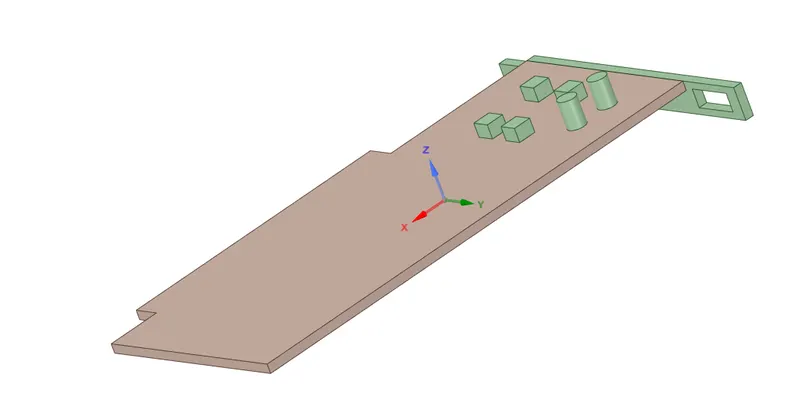
PART WISE DIAGRAMS:

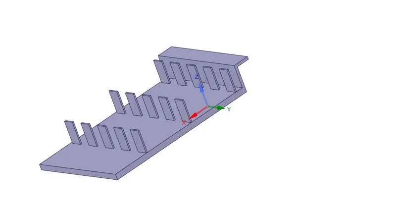
BASE	PROCESSOR AND COMPONENTS	FINS

MESHING:

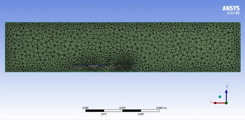
Fig. 2 Meshing for the Geometry

A baseline mesh (Element Size=`1e^(-2)`) was created for first case. And a refined mesh for the second (Element size=`2e^(-3)`). The respective faces were named Inlet, Outlet and Symmetry (Wind Tunnel Walls). The outer enclosure is hidden and the respective graphic card components are named individually.

SETUP:

Since the problelm statement is considered for a low Mach number, a Pressure Based Solver is considered for the simulation. The `k-epsilon` Standard Turbulence model was used for the respective test case calculations. A Steady State simulation is run. The Boundary condition for the Inlet (Velocity=3 m/s and Temperature=300K), Outlet (Static Pressure= 1 atm). The materials for the processor, base and fins of graphic card were chosen as Copper, Steel and Aluminium respectively. This was done by copying the materials in the solid domain from the Fluent Material Database. The Cellzones option was chosen wherein each component was selected and the respective material was assigned. The Processor Cell Zone was chosen and a source term was added. The power output from the processor is assumed to be `6W` for processor volume `64mm^3`. Hybrid Initialization is used for t=0 and 400 iterations were run for each case.

RESULTS:

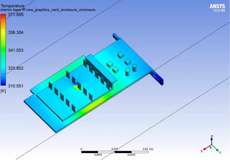
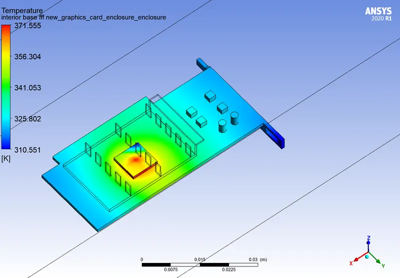
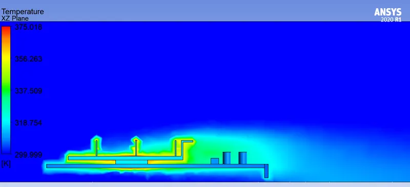
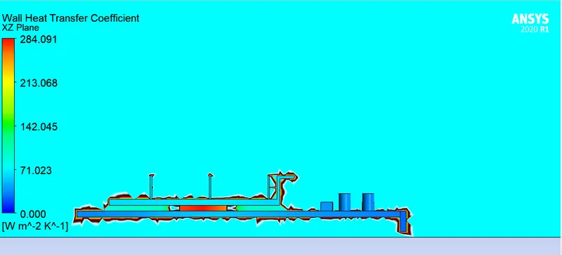
Comparing the Results for Mesh Dependency Test at 3m/s inlet air velocity:

Table 1: Comparison of Baseline and Refined Mesh Results

Output paramters	BASELINE MESH	REFINED MESH
Local Hotspot Region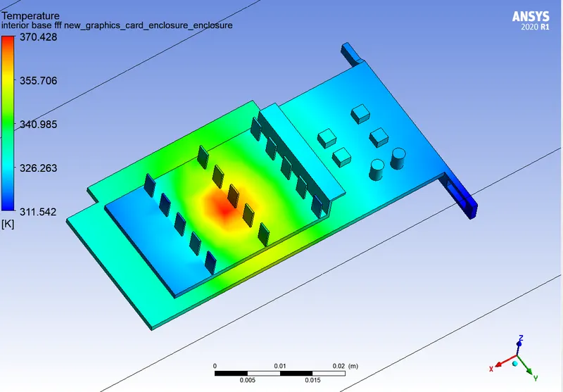
Local Processor Heat Dissipation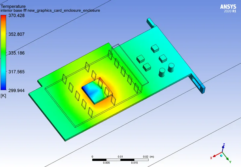
Local Temperature Contour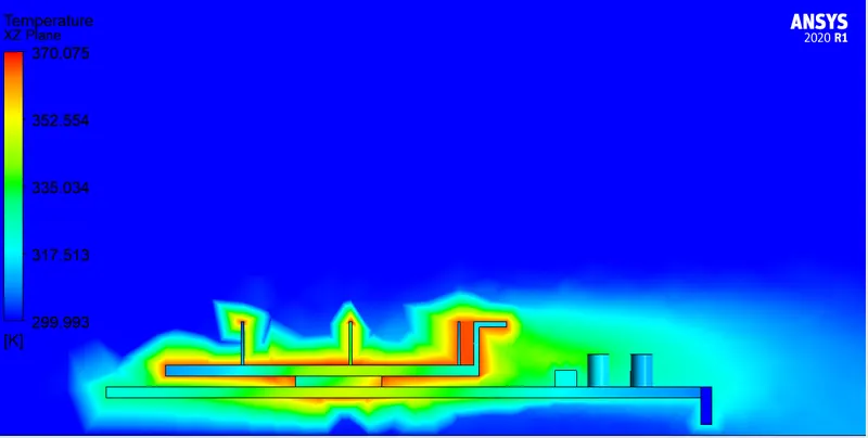
Wall Heat Transfer Coefficient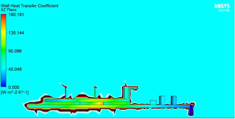
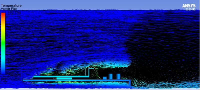
Vector Plot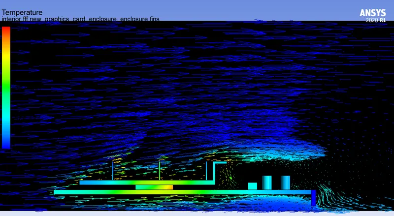

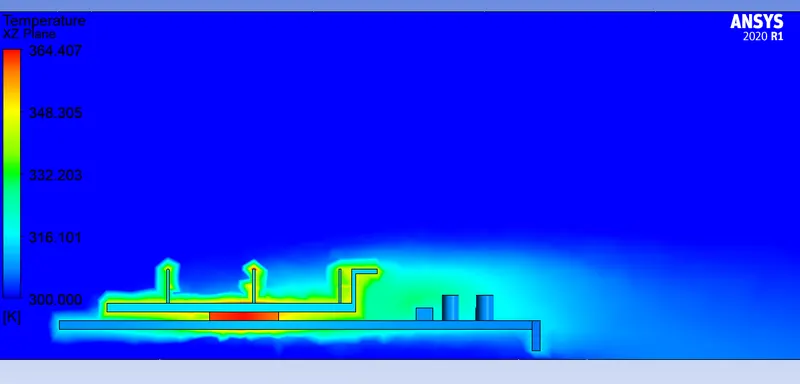
Comparison of Results at varied Velocities:

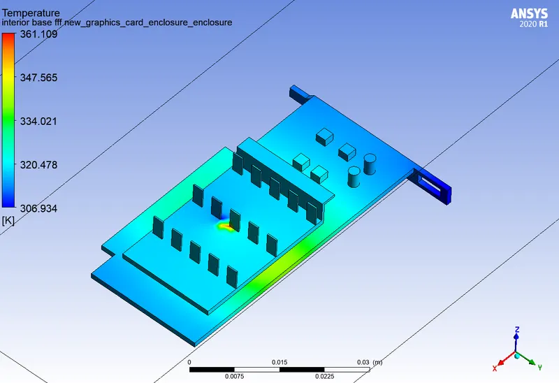
Table 2: Comparison of Results at various air inlet velocities

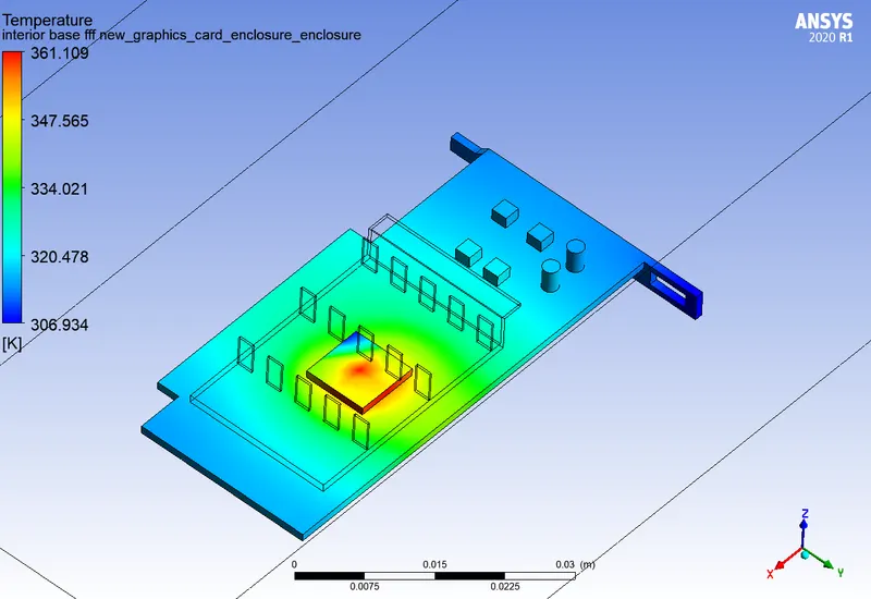
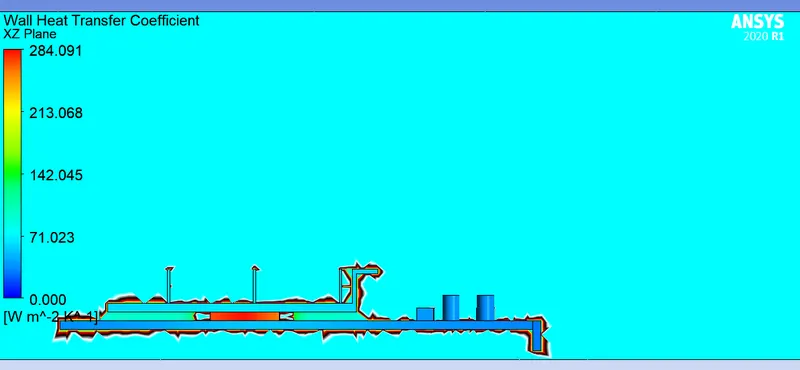
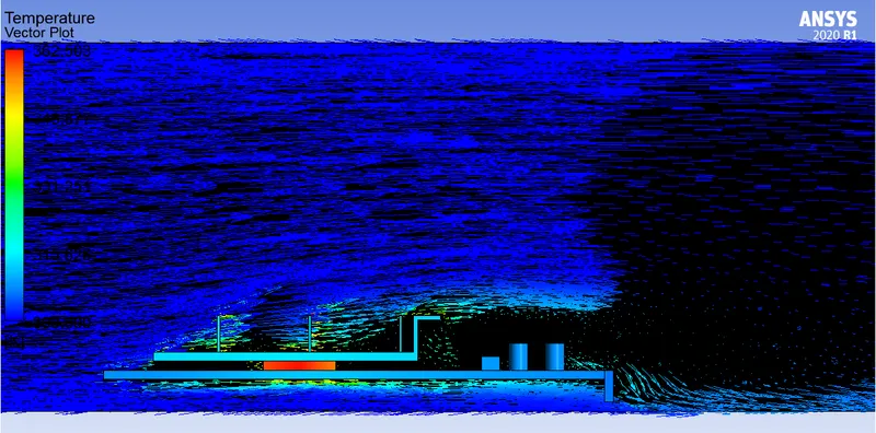
Output Paramters	Velocity=1 m/s	Veloctiy=5 m/s
Local Hotspot Region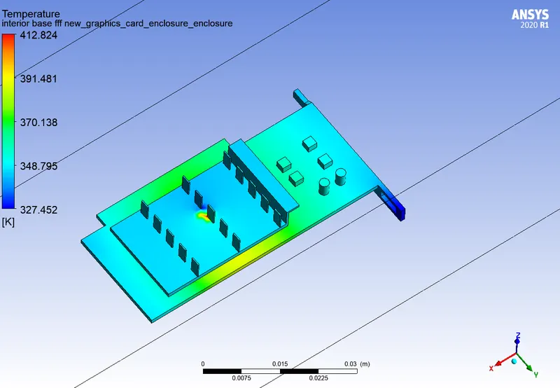
Local Processor Heat Dissipation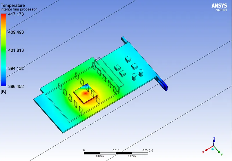
Local Temperature Contour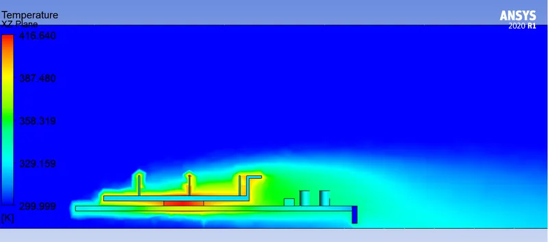
Wall Heat Transfer Coefficient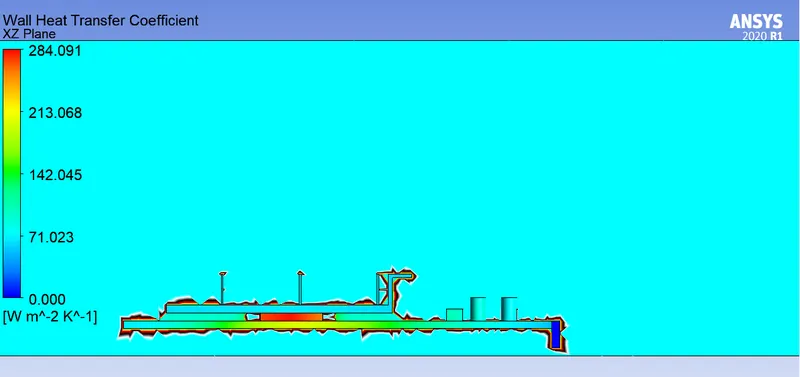
Vector Plot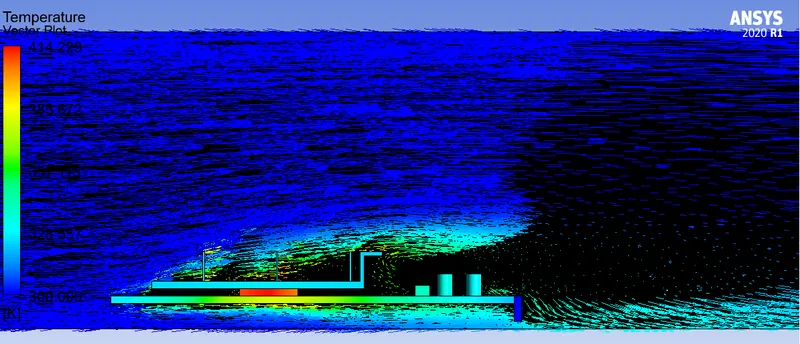

The tabulated results of all test cases are stated below:

Table 3: Maximum Temperature and Heat transfer Coefficient computations of all test cases

	Baseline Mesh	Refined Mesh
Velocity	3 m/s	1 m/s	3 m/s	5 m/s
Element Size	`1e^(-2)`	`2e^(-3)`	`2e^(-3)`	`2e^(-3)`
Surface Heat Transfer Coefficient (AWA) (Fluent) [`W/(m^2K)`]	26.949	15.839	28.853	34.564
Wall Adjacent Heat Transfer Coefficient (Fluent) (AWA) [`W/(m^2K)`]	65.203	86.730	86.627	87.192
Maximum Hotspot Temperature [`K`]	370.428	412.824	371.555	361.109
Maximum Contour Temperature [`K`]	370.075	416.640	375.018	364.407
Maximum Wall Heat Transfer Coeffieicnt (CFD Post)	180.191	284.091	284.091	284.091

Note: The Heat transfer coefficient computed in Fluent is for Aluminium fins only.

The Area Weighted Average (AWA) heat transfer coefficient is the calculation obtained in Fluent, where as the Maximum Heat Transfer Coefficient is obtained from CFD Post. The Surface Heat Transfer Coefficient should be considered for the baseline mesh and the Wall Adjacent Heat Transfer Coefficient for the Refined Mesh. This is because the Nearest Node Centroid was not applicable for the Baseline Mesh, and a standard reference value was used for `T_(ref)`. The adjacent wall heat transfer function gives the right computation in the refined mesh case as the `y^+` and the turbulence model add to the `T^+` computation giving the right heat transfer coefficient value.

To check for the convergence of the solution the residual plots and the report definition of Area Weighted Averaged Heat Transfer Coefficients are observed. The Convergence Check option in the Solution Tab in Fluent is turned off. This ensures that Fluent itself doesn't stop the simulation for previously set tolerance levels. Based on the plots and residuals the user gets to decide if the solution is acceptable or not. The solution is said to converge when the residual or heat transfer coefficient plots are showing stable values or steady fluctuations.

CONCLUSION:

The convective cooling was observed better at higher velocity for air inlet.

When the mesh was refined, the maximum graphic card temperature rised, as a finer mesh projected better heat transfer in the conjugate zones.

The better heat transfer showed a variation in the wall heat transfer coefficient (CFD Post). This wall heat transfer coefficient remained constant throughout all the refined mesh computations.

The vector plots shows the region of recirculation, where higher turbulenc eis experienced. In such cases, an additional refined enclosure is suggested in and around the graphic card and addition of inflation layers on the fin would explain the heat dissipation better.

Heat transfer coefficient is a function of the heat flux and temperature difference between the bodies. The temperature difference is again dependent on `T^+` and `y^+`. Therefore, the turbulence model and the `y^+` for the computation affect the heat transfer coefficient alot. Clearly the CFD Post HTC is not to be considered for calculations (Theoretical = `59-64W/(m^2K)`).