Curve fitting using PYTHON

CURVE FITTING USING PYTHON INBUILT FUNCTIONS

AIM:

• Write a code to fit a linear and cubic polynomial for the C_p
• Write a code to show split wise method for the same data.

GOVERNING EQUATIONS AND THEORY:

Curve Fitting is the principle used for formulation of a curve, closest to a dataset. The basic idea behind this principle is to create a polynomial function or relationship between the dependent and independent variables defining the dataset. This is also called Regression Analysis. In this analysis, based on the input dataset, a polynomial function is formulated and checked for best fit.

The calculation of the best fit is done by either of the four error parameters- The sum of squares due to the error (SSE), R-square, Adjusted R-squared, Root Mean Squared Error (RMSE). In the current problem statement R-squared error will be used. The description of the error and functions for calculation of the R-squared value is discussed in “BODY OF THE CONTENT”.

There exist two types of fits- Perfect and Best. Best Fit refers to the best possible fit the polynomial function can create to minimize errors. The Best Fit of a curve can be a Perfect Fit to the curve, but not vice-versa. Perfect Fit refers to a perfect curve with no errors completely overlapping with the original dataset.

For the calculation of R-squared:

correlation_matrix = np.corrcoef(cp, fit_cp)
correlation_xy = correlation_matrix[0,1]
r_squared = correlation_xy**2

The above code is used for the computation.

OBJECTIVES OF THE PROJECT:

• The main objective of the project is to use Python’s inbuilt functions and understand the regression analysis for a linear fit and a cubic fit.
• The original dataset will be plotted, and a linear regression fit will be formulated for it. Similarly, a cubic regression fit will be formulated and plotted to observe the error in the fit.
• An optimized solution to replicate the original dataset with lower order polynomial fit will be discussed and applied.

ANSWERS:

1. What does popt and pcov mean? (Watch the video to get some context)

A:

popt:array

Optimal values for the parameters so that the sum of the squared residuals of `func(temperature,^**popt)` is minimized.

pcov:2-D array

The estimated covariance of popt. The diagonals provide the variance of the parameter estimate. To compute one standard deviation errors on the parameters use `perr=text(np.sqrt(np.diag(pcov)))`.

2. What does np.array(temperature) do?

A:

The Numpy module is used to create a variable wherein the array of temperature values are stored. After the curve fit coefficients are computed, the the temperature array and coefficients should be input into the function to generate the curve fit specific heat values. But originally the functions are created to input single temperature value and output single specific heat value. An array input, gives out array of Cp values.

3. What does the * in *popt mean?

A:

Single asterisk as used in function declaration allows variable number of arguments passed from calling environment. Inside the function it behaves as a tuple. Therefore it acts as a pointer to the array popt, and multiple inputs can be given.

4. What needs to be done in order to make the curve fit perfect?

A:

Higher order curve fits ar shown (upto 5th). To fit it perfectly, the curve needs to be split, and then lower order curves can be used for each section. An example with cubic split wise fit is shown.

BODY OF THE CONTENT:

Code for linear regression:

import math
import matplotlib.pyplot as plt
import numpy as np
from scipy.optimize import curve_fit


#Curve Fit Function
def funclinear(t,a,b):
	return (a*t+b)
def funccubic(t,a,b,c,d):
	return (a*pow(t,3)+b*pow(t,2)+c*t+d)
def funcpoly(t,a,b,c,d,e,f):
	return (a*pow(t,5)+b*pow(t,4)+c*pow(t,3)+d*pow(t,2)+e*t+f)

#Function to read the data file and store the temperature and Cp values
def readfile():
	temp=[]
	cp=[]
	for line in open('data','r'):
		values=line.split(',')
		temp.append(float(values[0]))
		cp.append(float(values[1]))
	return [temp,cp]

#Input of the extracted data into variables
temperature,cp=readfile()
"""
#Using the curvefit function to extract coefficients for func polynomial

"""
LINEAR POLYNOMIAL FIT FOR DATASET
*********************************************************
"""
#Curve fit function to extract optimal coefficients for the desired polynomial
popt,pcov=curve_fit(funclinear,temperature,cp)
#Creating the new curve fit from the computed coefficients
fit_cp=funclinear(np.array(temperature),*popt)

#Plotting the original data and computed curve fit
plt.figure(1)
plt.plot(temperature,cp,color="blue",linewidth=3)
plt.plot(temperature,fit_cp,color="red",linewidth=3)
plt.legend(['Original Dataset','Linear Curve Fit'])
plt.xlabel('Temperature [K]')
plt.ylabel('Specific Heat Capacity [J/(mol.K)]')
plt.title('Curve Fit (1st Order)')
correlation_matrix = np.corrcoef(cp, fit_cp)
correlation_xy = correlation_matrix[0,1]
r_squared = correlation_xy**2
plt.text(2000, 1050, 'R-squared = %0.4f' % r_squared)

plt.savefig('linear')
plt.show()

"""
*********************************************************

"""

Explanation: The data is extracted from the 'data' file and stored in variables temperature and cp. The curve_fit function from the scipy module is employed to the linear function. The output coefficient popt is input into the function with the array of temperature values to generate the fitted curve. The results are plotted for comparison.

Output for linear regression:

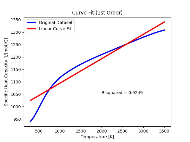
• For the linear curve fit, R²=0.925 is observed. To understand the curve fitting at higher polynomial orders a cubic fit is plotted in the next section.

Code for Cubic Fit:

"""
CUBIC POLYNOMIAL FIT FOR DATASET
*********************************************************
"""
#Curve fit function to extract optimal coefficients for the desired polynomial
popt,pcov=curve_fit(funccubic,temperature,cp)
#Creating the new curve fit from the computed coefficients
fit_cp=funccubic(np.array(temperature),*popt)

#Plotting the original data and computed curve fit
plt.figure(2)
plt.plot(temperature,cp,color="blue",linewidth=3)
plt.plot(temperature,fit_cp,color="red",linewidth=3)
plt.legend(['Original Dataset','Cubic Curve Fit'])
plt.xlabel('Temperature [K]')
plt.ylabel('Specific Heat Capacity [J/(mol.K)]')
plt.title('Curve Fit (3rd Order)')
correlation_matrix = np.corrcoef(cp, fit_cp)
correlation_xy = correlation_matrix[0,1]
r_squared = correlation_xy**2
plt.text(2000, 1050, 'R-squared = %0.4f' % r_squared)
plt.savefig('cubic')
plt.show()
"""
*********************************************************
"""

Output for Cubic Fit:

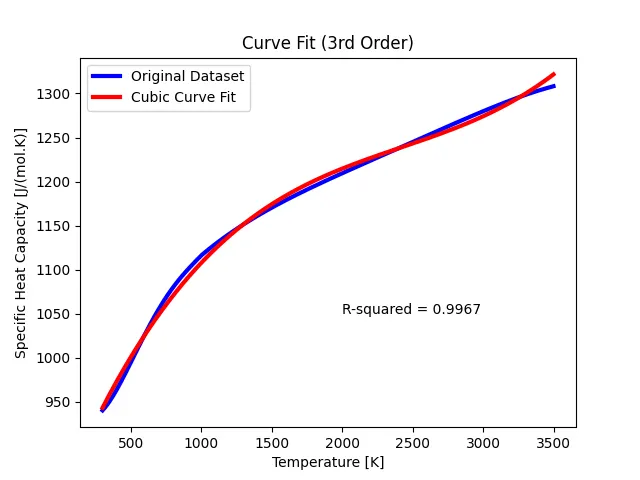
• For a cubic fit, R²=0.997 is observed. Therefore, explaining that the error is less and the cubic polynomial is a better fit for the dataset.

To improve the accuracy of the curve fit with the dataset, another higher order polynomial is computed at degree 5.

Code for a 5^th degree Polynomial Fit:

"""
FIFTH DEGREE POLYNOMIAL FIT FOR DATASET
*********************************************************
"""
#Curve fit function to extract optimal coefficients for the desired polynomial
popt,pcov=curve_fit(funcpoly,temperature,cp)
#Creating the new curve fit from the computed coefficients
fit_cp=funcpoly(np.array(temperature),*popt)

#Plotting the original data and computed curve fit
plt.figure(3)
plt.plot(temperature,cp,color="blue",linewidth=3)
plt.plot(temperature,fit_cp,color="red",linewidth=3)
plt.legend(['Original Dataset','Polynomial Curve Fit'])
plt.xlabel('Temperature [K]')
plt.ylabel('Specific Heat Capacity [J/(mol.K)]')
plt.title('Curve Fit (5th Order)')
correlation_matrix = np.corrcoef(cp, fit_cp)
correlation_xy = correlation_matrix[0,1]
r_squared = correlation_xy**2
plt.text(2000, 1050, 'R-squared = %0.4f' % r_squared)
plt.savefig('poly')
plt.show()
"""
**********************************************************
"""

Output for a 5^th degree Polynomial Fit:

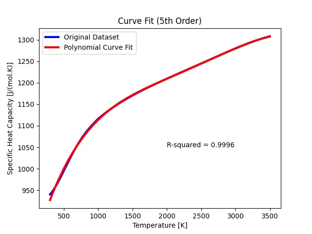
• It is observed that the R² value is increasing as the order of the polynomial is increased.
• To get a best fit, one can use either a very high order polynomial fit or split wise polynomial. Split wise polynomial works on the same principle as the curve fit used till now, but the dataset is distributed into sections and the curve fit is applied. More the number of sections, more accurately the respective curves can match the original dataset. And following this procedure, very high order polynomial function is not needed.

Split wise Polynomial:

• In this method, the original dataset is distributed into various number of sections, and the individually predicted C_p vectors are plotted against temperature. More the number of splits, more accurate is each respective polynomial.

Code for Cubic Split Wise Fit:

"""
CUBIC SPLIT WISE FIT POLYNOMIAL FOR DATASET
*********************************************************
"""
#To split the array of temperature and Cp, numpy module is used
array=np.array_split(temperature,3)
array2=np.array_split(cp,3)
temp1=array[0]
temp2=array[1]
temp3=array[2]
cp1=array2[0]
cp2=array2[1]
cp3=array2[2]
#Curve fit function to extract optimal coefficients for the desired polynomial
popt1,pcov1=curve_fit(funccubic,temp1,cp1)
popt2,pcov2=curve_fit(funccubic,temp2,cp2)
popt3,pcov3=curve_fit(funccubic,temp3,cp3)
#Creating the new curve fit from the computed coefficients
fit_cp1=funccubic(np.array(temp1),*popt1)
fit_cp2=funccubic(np.array(temp2),*popt2)
fit_cp3=funccubic(np.array(temp3),*popt3)
#Plotting the original data and computed curve fit
plt.figure(4)
plt.plot(temperature,cp,color="black",linewidth=3)
plt.plot(temp1,fit_cp1,color="red",linewidth=3)
plt.plot(temp2,fit_cp2,color="blue",linewidth=3)
plt.plot(temp3,fit_cp3,color="green",linewidth=3)
plt.legend(['Original Dataset','Cubic Curve Fit 1','Cubic Curve Fit 2','Cubic Curve Fit 3'])
plt.xlabel('Temperature [K]')
plt.ylabel('Specific Heat Capacity [J/(mol.K)]')
plt.title('Split Wise Cubic Curve Fit (3rd Order)')
plt.savefig('split')
plt.show()

"""
*********************************************************
"""

Output for Cubic Split wise Fit:

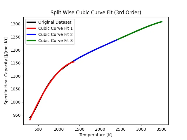
• It is observed that the section wise R² value of the Cubic fit has increased, leading to a much better fit to the original dataset.

CONCLUSION:

• The 1^st Order Polynomial fit gives the least `R^2` value when compared with the original dataset.
• As the degree of the polynomial is increased the error is reducing and the curve fits better than the lower degree polynomials.
• To improve the curve at a lower degree polynomial fit, split wise polynomial fit is used. This method ensures section wise accuracy, without the need to increase the order of the polynomial.
• The R-squared value for section 1 in the Split wise polynomial fit is comparitively lower than the other sections. This can be inproved by solely increasing splits/increasing number of sections in the 1st section.