Curve Fitting using MATLAB

CURVE FITTING USING MATLAB INBUILT FUNCTIONS

AIM:

• Write a code to fit a linear and cubic polynomial for the C_p
• Write a code to show split wise method for the same data.

GOVERNING EQUATIONS AND THEORY:

Curve Fitting is the principle used for formulation of a curve, closest to a dataset. The basic idea behind this principle is to create a polynomial function or relationship between the dependent and independent variables defining the dataset. This is also called Regression Analysis. In this analysis, based on the input dataset, a polynomial function is formulated and checked for best fit.

The calculation of the best fit is done by either of the four error parameters- The sum of squares due to the error (SSE), R-square, Adjusted R-squared, Root Mean Squared Error (RMSE). In the current problem statement R-squared error will be used. The description of the error and functions for calculation of the R-squared value is discussed in “BODY OF THE CONTENT”.

There exist two types of fits- Perfect and Best. Best Fit refers to the best possible fit the polynomial function can create to minimize errors. The Best Fit of a curve can be a Perfect Fit to the curve, but not vice-versa. Perfect Fit refers to a perfect curve with no errors completely overlapping with the original dataset.

For the calculation of R-squared:
`R^2=[(SS.nr)/(||C_p-mean(C_p)||)]^2`

where nr is the normr function to normalize the structure SS obtained from the polyfit command explained in the later sections.

OBJECTIVES OF THE PROJECT:

• The main objective of the project is to use MATLAB’s inbuilt functions and understand the regression analysis for a linear fit and a cubic fit.
• The original dataset will be plotted, and a linear regression fit will be formulated for it. Similarly, a cubic regression fit will be formulated and plotted to observe the error in the fit.
• An optimized solution to replicate the original dataset with lower order polynomial fit will be discussed and applied.

BODY OF THE CONTENT:

Explanation of the CODE:

• The program is coded in MATLAB. Initially a data file is used to input the Specific Heat vs Temperature dataset into the MATLAB workspace. “load” command is used to input the data.
• The temperature and specific heat values are separated and input into various column vectors.
• “polyfit” command is used to create the coefficients of an n^th order polynomial from the original dataset; [coefficient]=polyfit(x,y,n). The ‘polyval’ command is used to create a vector calculating the y-coordinate of the function using the computed coefficients and the input temperature (x-coordinates).

• First, the original dataset is plotted and a linear regression curve is computed.

Code for linear regression:

clear all
close all
clc
%Program for curve fitting of a dataset using MATLAB inbuilt functions
%The original dataset is between specific heat and temperature
%load is command is used to extract the two vectors from file 'data'
%and enter into cp_data matrix
cp_data=load('data');
%cp_data is 3200x2 dataset, in which 1st row represents temperature
%and 2nd row represents cp values
%The respective row datas are assigned to temp and cp, two column vectors
temp=cp_data(:,1);
cp=cp_data(:,2);
%polyfit command is used to create coefficients for the curve fit
%polynomial of degree '1'. These coefficients are input into the vector
%coeff. SS and mu are vectors added for the rectification of centering and 
%scaling error encountered at higher orders of polynomial fit.
[coeff,SS,mu]=polyfit(temp,cp,1);
%R-squared value for the curve is plotted using the SS structure output
%from polyfit command. R-squared is a measure of the error of the plot with
%respect to the original dataset
r2=1-(SS.normr/norm(cp-mean(cp)))^2;
%The predicted y-coordinates/cp values are formulated using polyval command
predicted_cp=polyval(coeff,temp,SS,mu);
%The original dataset and predicted dataset are plotted and the R-squared
%value is compared
hold on
plot(temp,predicted_cp,'color','r','linewidth',3)
plot(temp,cp,'color','b','linewidth',3)
text(2500,1050,sprintf('R^2= %g',r2))
legend('Curve Fit Polynomial','Original Dataset')
xlabel('Temperature [K]')
ylabel('Specific Heat [kJ/kmol-K]')
title('Curve Fit (1st Order)')

• The same procedure as explained above is coded. The R² is calculated and input on the plot below.

Output for linear regression:

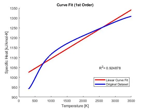
• For the linear curve fit, R²=0.925 is observed. To understand the curve fitting at higher polynomial orders a cubic fit is plotted in the next section.

Code for Cubic Fit:

clear all
close all
clc
%Program for curve fitting of a dataset using MATLAB inbuilt functions
%The original dataset is between specific heat and temperature
%load is command is used to extract the two vectors from file 'data'
%and enter into cp_data matrix
cp_data=load('data');
%cp_data is 3200x2 dataset, in which 1st row represents temperature
%and 2nd row represents cp values
%The respective row datas are assigned to temp and cp, two column vectors
temp=cp_data(:,1);
cp=cp_data(:,2);
%polyfit command is used to create coefficients for the curve fit
%polynomial of degree '3'. These coefficients are input into the vector
%coeff. SS and mu are vectors added for the rectification of centering and 
%scaling error encountered at higher orders of polynomial fit.
[coeff,SS,mu]=polyfit(temp,cp,3);
%R-squared value for the curve is plotted using the SS structure output
%from polyfit command. R-squared is a measure of the error of the plot with
%respect to the original dataset
r2=1-(SS.normr/norm(cp-mean(cp)))^2;
%The predicted y-coordinates/cp values are formulated using polyval command
predicted_cp=polyval(coeff,temp,SS,mu);
%The original dataset and predicted dataset are plotted and the R-squared
%value is compared
hold on
plot(temp,predicted_cp,'color','r','linewidth',3)
plot(temp,cp,'color','b','linewidth',3)
text(2500,1050,sprintf('R^2= %g',r2))
legend('Curve Fit Polynomial','Original Dataset')
xlabel('Temperature [K]')
ylabel('Specific Heat [kJ/kmol-K]')
title('Curve Fit (3rd Order)')

Output for Cubic Fit:

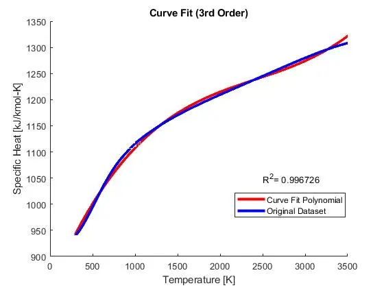
• For a cubic fit, R²=0.997 is observed. Therefore, explaining that the error is less and the cubic polynomial is a better fit for the dataset. But the following error was observed for the code of cubic fit:

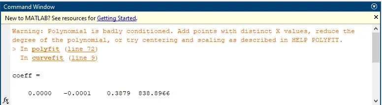
To rectify this an output vector SS was used. The ‘SS’ added to the output vector ([coeff,SS,mu]=polyfit(x,y,3)) refers to structure. The coefficients formulated for the best fit of the polynomial are added in the vector [coefficients]. The structure created ‘SS’, contains fields R, df and normr referring to the triangular factor from a QR decomposition of the Vandermonde matrix of x, the degrees of freedom, and the norm of the residuals, respectively. ’mu’ is a 2 element vector which contains the centring and scaling values. In mu, mu(1) is mean(x) and mu(2) is std(x). Using these polyfit centers x at 0 and scales to have unit standard deviation.

To improve the accuracy of the curve fit with the dataset, another higher order polynomial is computed at degree 5.

Code for a 5^th degree Polynomial Fit:

clear all
close all
clc
%Program for curve fitting of a dataset using MATLAB inbuilt functions
%The original dataset is between specific heat and temperature
%load is command is used to extract the two vectors from file 'data'
%and enter into cp_data matrix
cp_data=load('data');
%cp_data is 3200x2 dataset, in which 1st row represents temperature
%and 2nd row represents cp values
%The respective row datas are assigned to temp and cp, two column vectors
temp=cp_data(:,1);
cp=cp_data(:,2);
%polyfit command is used to create coefficients for the curve fit
%polynomial of degree '5'. These coefficients are input into the vector
%coeff. SS and mu are vectors added for the rectification of centering and 
%scaling error encountered at higher orders of polynomial fit.
[coeff,SS,mu]=polyfit(temp,cp,5);
%R-squared value for the curve is plotted using the SS structure output
%from polyfit command. R-squared is a measure of the error of the plot with
%respect to the original dataset
r2=1-(SS.normr/norm(cp-mean(cp)))^2;
%The predicted y-coordinates/cp values are formulated using polyval command
predicted_cp=polyval(coeff,temp,SS,mu);
%The original dataset and predicted dataset are plotted and the R-squared
%value is compared
hold on
plot(temp,predicted_cp,'color','r','linewidth',3)
plot(temp,cp,'color','b','linewidth',3)
text(2500,1050,sprintf('R^2= %g',r2))
legend('Curve Fit Polynomial','Original Dataset')
xlabel('Temperature [K]')
ylabel('Specific Heat [kJ/kmol-K]')
title('Curve Fit (5th Order)')

Output for a 5^th degree Polynomial Fit:

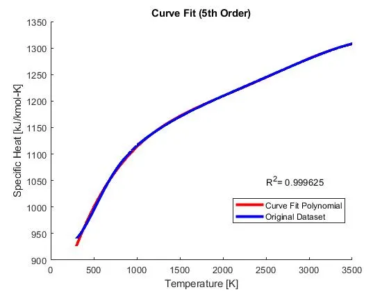
• It is observed that the R² value is increasing as the order of the polynomial is increased.
• To get a best fit, one can use either a very high order polynomial fit or split wise polynomial. Split wise polynomial works on the same principle as the curve fit used till now, but the dataset is distributed into sections and the curve fit is applied. More the number of sections, more accurately the respective curves can match the original dataset. And following this procedure, very high order polynomial function is not needed.

Split wise Polynomial:

• In this method, the original dataset is distributed into various number of sections, and the individually predicted C_p vectors are plotted against temperature. More the number of splits, more accurate is each respective polynomial.

Code for Cubic Split Wise Fit:

clear all
close all
clc
%Program for curve fitting of a dataset using MATLAB inbuilt functions
%The original dataset is between specific heat and temperature
%load is command is used to extract the two vectors from file 'data'
%and enter into cp_data matrix
cp_data=load('data');
%cp_data is 3200x2 dataset, in which 1st row represents temperature
%and 2nd row represents cp values
%The respective row datas are assigned to temp and cp, two column vectors
temp=cp_data(:,1);
cp=cp_data(:,2);
%The sections of the datset are divided into 1,2,and 3. And the respective
%data values are assigned to the vectors. The procedure is same.
cp1=cp(1:1100);
temp1=temp(1:1100);
cp2=cp(1101:2200);
temp2=temp(1101:2200);
cp3=cp(2201:3200);
temp3=temp(2201:3200);
%polyfit command is used to create coefficients for the curve fit
%polynomial of degree '5'. These coefficients are input into the vector
%coeff. SS and mu are vectors added for the rectification of centering and 
%scaling error encountered at higher orders of polynomial fit.
[coeff1,SS1,mu1]=polyfit(temp1,cp1,3);
[coeff2,SS2,mu2]=polyfit(temp2,cp2,3);
[coeff3,SS3,mu3]=polyfit(temp3,cp3,3);
%R-squared value for the curve is plotted using the SS structure output
%from polyfit command. R-squared is a measure of the error of the plot with
%respect to the original dataset
r1=1-(SS1.normr/norm(cp1-mean(cp1)))^2;
r2=1-(SS2.normr/norm(cp2-mean(cp2)))^2;
r3=1-(SS3.normr/norm(cp3-mean(cp3)))^2;
%The predicted y-coordinates/cp values are formulated using polyval command
predicted_cp1=polyval(coeff1,temp1,SS1,mu1);
predicted_cp2=polyval(coeff2,temp2,SS2,mu2);
predicted_cp3=polyval(coeff3,temp3,SS3,mu3);
%The original dataset and predicted dataset are plotted and the R-squared
%value is compared
hold on
plot(temp1,predicted_cp1,'color','r','linewidth',4)
plot(temp2,predicted_cp2,'color','b','linewidth',4)
plot(temp3,predicted_cp3,'color','g','linewidth',4)
plot(temp,cp,'color',[0 0 0],'linewidth',1.5)
text(500,1200,sprintf('R^2= %g',r1))
text(1750,1300,sprintf('R^2= %g',r2))
text(2750,1200,sprintf('R^2= %g',r3))
legend('Curve Fit Section 1','Curve Fit Section 2','Curve Fit Section 3','Original Dataset')
xlabel('Temperature [K]')
ylabel('Specific Heat [kJ/kmol-K]')
title('Curve Fit (3rd Order)- Split wise')

Output for Cubic Split wise Fit:

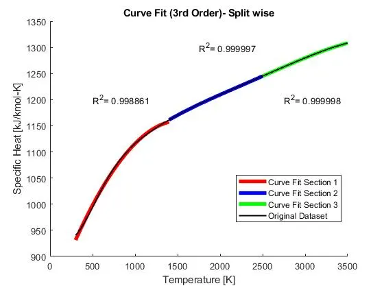
• It is observed that the section wise R² value of the Cubic fit has increased, leading to a much better fit to the original dataset.

CONCLUSION:

• The 1^st Order Polynomial fit gives the least R² value when compared with the original dataset.
• As the degree of the polynomial is increased the error is reducing and the curve fits better than the lower degree polynomials.
• To improve the curve at a lower degree polynomial fit, split wise polynomial fit is used. This method ensures section wise accuracy, without the need to increase the order of the polynomial.
• The R-squared value for section 1 in the Split wise polynomial fit is comparitively lower than the other sections. This can be inproved by solely increasing splits/increasing number of sections in the 1st section.

REFERENCES:

• https://in.mathworks.com/help/matlab/ref/polyfit.html
• https://www.mathworks.com/matlabcentral/answers/159369-polyfit-and-r-2-value
• https://in.mathworks.com/matlabcentral/answers/157183-polyfit-with-centering-and-scaling-values
• Introduction to Curve Fitting, NCSS Statistical Software:https://ncss-wpengine.netdna-ssl.com/wp-content/themes/ncss/pdf/Procedures/NCSS/Introduction_to_Curve_Fitting.pdf