SOLVING STEADY AND UNSTEADY 2D HEAT CONDUCTION PROBLEM

AIM:

• Solve for the steady state and transient analysis of the 2D heat conduction equation.
• For each case, program a MATLAB code using Jacobi, Gauss Seidel and Successive Over Relaxation (SOR) method.
• Consider the cases of explicit and implicit solution for each sub-case and show results.

OBJECTIVES OF THE PROJECT:

• Derive the general equation for steady state analysis using central differencing scheme in space and apply the Jacobi, Gauss Seidel and SOR method to compute the numerical equation.
• Derive the general equation for transient state using central differncing scheme in space and forward differencing scheme in time. Apply the respective notations based on the solving method and compute the numerical equation.
• Derive the implicit and explicit solution for the transient analysis and derive the Jacobi, Gauss Seidel and SOR method equations.
• Solve the iterative solutions and produce the output observed at final iteration.

GOVERNING EQUATIONS AND THEORY:

• The 3 Dimensional Heat conduction equation is expressed as:
• `(delT)/(delt)=α((del^2T)/(delx^2)+(del^2T)/(dely^2)+(del^2T)/(delz^2))`
• when reduced to 2 dimensions, the z-derivative is elimiated:
• `(delT)/(delt)=α((del^2T)/(delx^2)+(del^2T)/(dely^2))`
• For solving the two problem statements- In steady state the time derivative term is eliminated and in transient state the time derivative term is considered.

• STEADY STATE:
• The equation reduces to:
• `((del^2T)/(delx^2)+(del^2T)/(dely^2))=0`
• To solve the equation, data points from both left and right of the derivative point is required. And this being a 2D problem, the top and bottom grid data points are also used for accurate numerical solution.
• Therefore,using the central differencing for second derivative on each term:
• `(T_(i+1,j)−2T_(i,j)+T_(i−1,j))/(Deltax^2)+(T_(i,j−1)−2T_(i,j)+T_(i,j+1))/(Deltay^2)=0`
• where `i` and `j` represent the x and y grid point respectively. Solving for the solution at `T_(i,j)`, the following equation is derived:
• `T_(i,j)=(Deltax^2.Deltay^2)/(2(Deltax^2+Deltay^2))((T_(i+1,j)+T_(i−1,j))/(Deltax^2)+(T_(i,j−1)+T_(i,j+1))/(Deltay^2))`_____(1)
• The above equation is used in the computation of steady state solutions.

• To apply the Jacobi method for this computation all the old values are used for the computation of the new `T_(i,j)`:
• `T_(i,j)^(n+1)=(Deltax^2.Deltay^2)/(2(Deltax^2+Deltay^2))((T_(i+1,j)^n+T_(i−1,j)^n)/(Deltax^2)+(T_(i,j−1)^n+T_(i,j+1)^n)/(Deltay^2))`
• where nn refers to the temperature data in the previous time step and `n+1` refers to the temperature data in the current time step, of which the computation is being carried out.

• For the computation of numerical solution using Gauss Seidel method the new termperature values are used of the already computed points. As the loop runs from `i`, 1 to number of grid points and `j`, 1 to number of grid points, at `T_(i,j)`,`T_(i-1,j)` and `T_(i,j-1)` are already computed, and these updated values can be used in the current computation:
• `T_(i,j)^(n+1)=(Deltax^2.Deltay^2)/(2(Deltax^2+Deltay^2))((T_(i+1,j)^n+T_(i−1,j)^(n+1))/(Deltax^2)+(T_(i,j−1)^(n+1)+T_(i,j+1)^n)/(Deltay^2))`

• To apply the SOR method on the Gauss Seidel computation, a factor `omega` is used. Based on the value of this factor, if `omega>1`, the solution converges faster, if `omega<1` the solution converges slower. the faster and slower is in comparison with the numerical solution being improved, either Gauss Seidel or Jacobi:
• `T_(SOR)^(n+1)=ωT_(GS)^(n+1)+(1−ω)T_(i,j)^n`

TRANSIENT ANALYSIS:

Transient Analysis includes the time derivative term in the 2D heat conduction equation. The similar procedure of central differencing is applied on the space derivatives and a forward differencing is applied on the time derivative:

`(delT)/(delt)=α((del^2T)/(delx^2)+(del^2T)/(dely^2))`

`(T_(i,j)^(n+1)−T_(i,j)^n)/(Deltat)=alpha((T_(i−1,j)^x−2T_(i,j)^x+T_(i+1,j)^x)/(Deltax^2)+(T_(i,j−1)^x−2T_(i,j)^x+T_(i,j+1)^x)/(Deltay^2))`

where `x` is prescribed `n` for explicit solution and `n+1` for implicit solution. In explicit solution only one unknown element in the equation exists `T_(i,j)^(n+1)` therefore a simple 2D loop, with a constant comparison with the previous time step solution is run to reach the steady state solution. In the implicit case, the number of unknown elements are more. Therefore, the unknown parameters are initially guessed. And for each time step another error calculation loop is run to check whether the solution for each time step is converging or not.

Explicit Solution:

The following equation is used to express the explicit solution for the transient equation:

`(T_(i,j)^(n+1)−T_(i,j)^n)/(Deltat)=alpha((T_(i−1,j)^n−2T_(i,j)^n+T_(i+1,j)^n)/(Deltax^2)+(T_(i,j−1)^n−2T_(i,j)^n+T_(i,j+1)^n)/(Deltay^2))`

Solving for `T_(i,j)^(n+1)`:

`T_(i,j)^(n+1)=T_(i,j)^n+alphaDeltat((T_(i−1,j)^n−2T_(i,j)^n+T_(i+1,j)^n)/(Deltax^2)+(T_(i,j−1)^n−2T_(i,j)^n+T_(i,j+1)^n)/(Deltay^2))`

Explicit method is useful as the code is simple, but when taken for a higher number of grid points and in 3D space the computation time is much higher.

Implicit Solution:

The following equation is used to express the implicit solution for the transient equation:

`(T_(i,j)^(n+1)−T_(i,j)^n)/(Deltat)=alpha((T_(i−1,j)^(n+1)−2T_(i,j)^(n+1)+T_(i+1,j)^(n+1))/(Deltax^2)+(T_(i,j−1)^(n+1)−2T_(i,j)^(n+1)+T_(i,j+1)^(n+1))/(Deltay^2))`

Solving for `T_(i,j)^(n+1)`:

`T_(i,j)^(n+1)=T_(i,j)^n+alphaDeltat((T_(i−1,j)^(n+1)−2T_(i,j)^(n+1)+T_(i+1,j)^(n+1))/(Deltax^2)+(T_(i,j−1)^(n+1)−2T_(i,j)^(n+1)+T_(i,j+1)^(n+1))/(Deltay^2))`

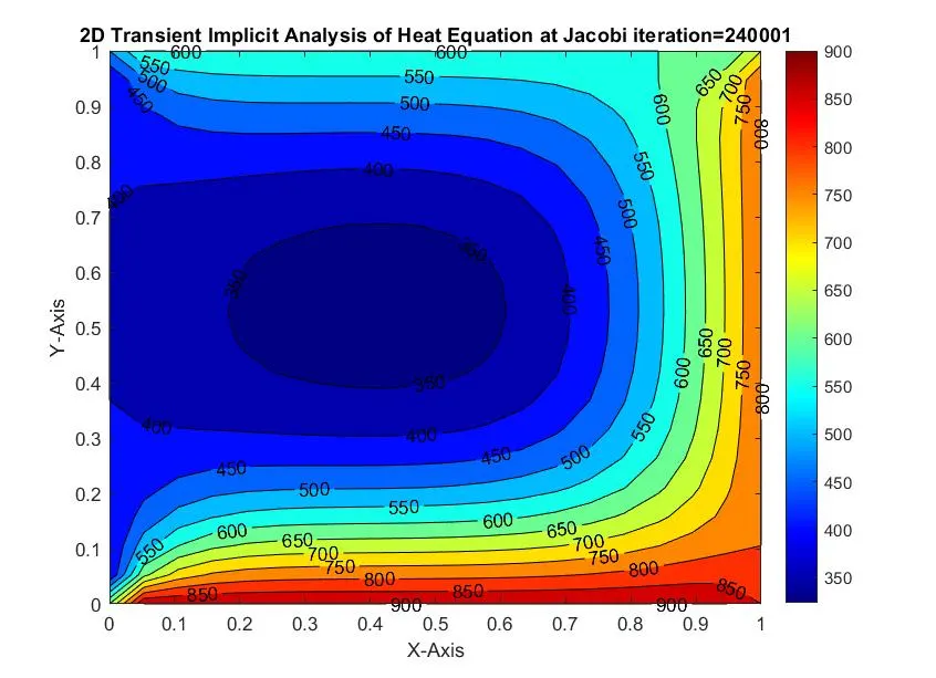
In Jacobi method for the implicit solution, an initial condition temperature matrix is input. In each time loop, an error comparison is done with the previous solution matrix, and the loop is repated at the same time frame until the solution converges and minimal error solution is obtained. Now, this is stored as the previous time steps data and the next time step solution is computed till convergence is reached. Therefore, all the `n+1` time step temperature values on the RHS are assumed to be the old values similar to previous time step, and the space loop for x and y is run till convergence is reached.

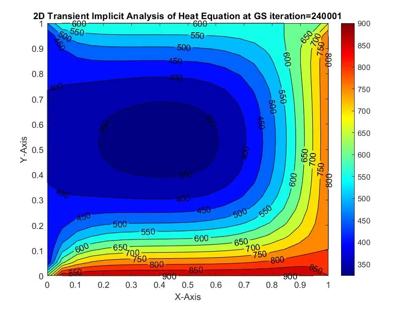
As in the steady state case for the Gauss Seidel method, the implicit case also updates the already computed values of `T_(i−1,j)^(n+1)` and `T_(i,j−1)^(n+1)`. Therefore the new values of the mentioned temperature values are input and old values of the other values. This is similarly run on time loop and another while loop inside till convergence is reached.

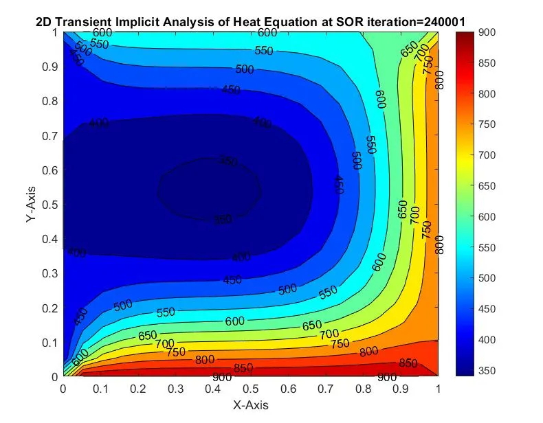
In the SOR method for the improvement of Gauss Seidel method, the computed temperature value using the GS method is input inot the SOR formula:

`T_(SOR)^(n+1)=ωT_(GS)^(n+1)+(1−ω)T_(i,j)^n`

BODY OF THE CONTENT:

STEADY STATE SOLUTION:

%Steady state 2D Temperature Heat Conduction Equation  
clear all,close all,clc
%The number of nodes on each axes are defined
nx=10;
ny=nx;
%The grid is divided based on number of nodes
x=linspace(0,1,nx);
y=linspace(0,1,ny);
dx=x(2)-x(1);
dy=y(2)-y(1);
%A mesh(2D matrix) is created based on the x and y coordinates of axes
[xx,yy]=meshgrid(x,y);
%Boundary Conditions
T=ones(nx,ny);
T(1,:)=900;
T(end,:)=600;
T(:,1)=400;
T(:,end)=800;
%The initial values are input in Told for calculation of next time step
Told=T;
%the tolerance error and initial error ar einput
error_tol=1e-4;
initial_error=9e9;
%Solver number is input for the respective method's function 
iterative_solver=1;
%Conditional statements are input based on the iterative_solver value 
%for each computation 
if iterative_solver==1
    Tjacobi=jacobi_steady_state(dx,dy,T,Told,xx,yy,nx,ny,initial_error,error_tol);
else if iterative_solver==2
    Tgauss=gauss_steady_state(dx,dy,T,Told,xx,yy,nx,ny,initial_error,error_tol);
else if iterative_solver==3
    Tsor=sor_steady_state(dx,dy,T,Told,xx,yy,nx,ny,initial_error,error_tol);
end    
    end
end

FUNCTION FOR JACOBI METHOD:

%Function to solve 2D steady state heat conduction equation using Jacobi method
function [T]=jacobi_steady_state(dx,dy,T,Told,xx,yy,nx,ny,comp_error,error_tol)
   %Iteration number is set to 1  
   jacobi_iter=1;
   %constant computed based on derived equation of the solver solution
   k=(dx^2*dy^2)/(2*(dx^2+dy^2));
   %A while loop is run for the convergence of solution based on error
   while(comp_error>error_tol)
       %Space loops in x and y are run for the computation of solution
       for i=2:nx-1
          for j=2:ny-1
              term1=(k*(Told(i+1,j)+Told(i-1,j)))/(dx^2);
              term2=(k*(Told(i,j+1)+Told(i,j-1)))/(dy^2);
              T(i,j)=term1+term2;
          end    
       end 
       %Error is calculated, and when it is higher than tolerance error, 
       %the loop repeats 
       comp_error=max(max(abs(Told-T)));
       %Told refers to the previous iteration values and are updated after
       %each loop
       Told=T;
       jacobi_iter=jacobi_iter+1;
       %Plotting of 2D output
       figure(1)
       [a,b]=contourf(xx,yy,T);
       colormap(jet)
       colorbar
       title(sprintf('Jacobi iteration number=%d for steady state',jacobi_iter))
       xlabel('X-Axis')
       ylabel('Y-Axis')
       clabel(a,b)
       pause(0.05)
   end    
end

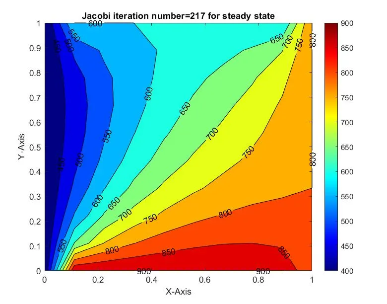
OUTPUT FOR JACOBI METHOD:

FUNCTION FOR GAUSS SEIDEL METHOD:

%Function to solve 2D steady state heat conduction equation using GS method
function [T]=gauss_steady_state(dx,dy,T,Told,xx,yy,nx,ny,comp_error,error_tol)
   %Iteration number is set to 1  
   gauss_iter=1;
   %constant computed based on derived equation of the solver solution
   k=(dx^2*dy^2)/(2*(dx^2+dy^2));
   %A while loop is run for the convergence of solution based on error
   while(comp_error>error_tol)
       %Space loops in x and y are run for the computation of solution
       for i=2:nx-1
          for j=2:ny-1
              term1=(k*(Told(i+1,j)+T(i-1,j)))/(dx^2);
              term2=(k*(Told(i,j+1)+T(i,j-1)))/(dy^2);
              T(i,j)=term1+term2;
          end    
       end 
       %Error is calculated, and when it is higher than tolerance error, 
       %the loop repeats 
       comp_error=max(max(abs(Told-T)));
       %Told refers to the previous iteration values and are updated after
       %each loop
       Told=T;
       gauss_iter=gauss_iter+1;
       %Plotting of 2D output
       figure(1)
       [a,b]=contourf(xx,yy,T);
       colormap(jet)
       colorbar
       title(sprintf('Gauss Seidel iteration number=%d for steady state',gauss_iter))
       xlabel('X-Axis')
       ylabel('Y-Axis')
       clabel(a,b)
       pause(0.05)
   end    
end

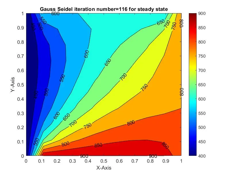
OUTPUT FOR GAUSS SEIDEL METHOD:

FUNCTION FOR SOR METHOD:

%Function to solve 2D steady state heat conduction equation using SOR
%method on GS solver
function [T]=sor_steady_state(dx,dy,T,Told,xx,yy,nx,ny,comp_error,error_tol)
   %Iteration number is set to 1
   sor_iter=1;
   %A relaxation constant is input for the solver
   omega=1.2;
   %constant computed based on derived equation of the solver solution
   k=(dx^2*dy^2)/(2*(dx^2+dy^2));
   %A while loop is run for the convergence of solution based on error
   while(comp_error>error_tol)
       %Space loops in x and y are run for the computation of solution
       for i=2:nx-1
          for j=2:ny-1
              term1=(k*(Told(i+1,j)+T(i-1,j)))/(dx^2);
              term2=(k*(Told(i,j+1)+T(i,j-1)))/(dy^2);
              P=term1+term2;
              T(i,j)=omega*P+(1-omega)*Told(i,j);
          end    
       end 
       %Error is calculated, and when it is higher than tolerance error, 
       %the loop repeats 
       comp_error=max(max(abs(Told-T)));
       %Told refers to the previous iteration values and are updated after
       %each loop
       Told=T;
       sor_iter=sor_iter+1;
       %Plotting of 2D output
       figure(1)
       [a,b]=contourf(xx,yy,T);
       colormap(jet)
       colorbar
       title(sprintf('SOR iteration number=%d for steady state',sor_iter))
       xlabel('X-Axis')
       ylabel('Y-Axis')
       clabel(a,b)
       pause(0.05)
   end    
end

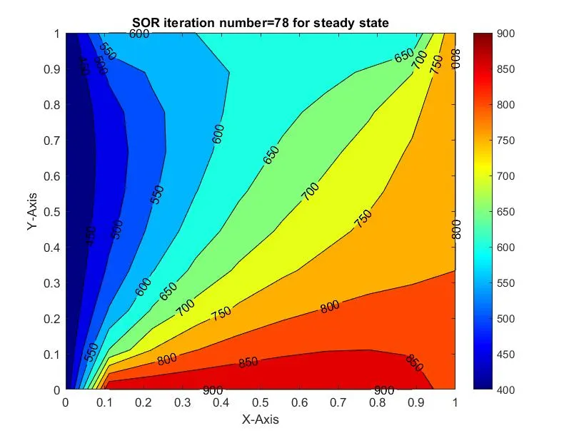
OUTPUT FOR SOR METHOD:

TRANSIENT STATE EXPLICIT SOLUTION:

%2D Temperature Transient Heat Conduction Equation solved explicitly 
clear all,close all,clc
%The number of nodes on each axis are defined
nx=20;
ny=nx;
%The node distance is defined based on number of nodes
x=linspace(0,1,nx);
y=linspace(0,1,ny);
dx=x(2)-x(1);
dy=y(2)-y(1);
%Time step for the computation is input
dt=0.01;
%Thermal diffusivity of air is input
alpha=1.9e-5;
%A mesh(2D Matrix) is created based on the grid node values in each axis
[xx,yy]=meshgrid(x,y);
%Boundary Conditions
T=ones(nx,ny);
T(1,:)=900;
T(end,:)=600;
T(:,1)=400;
T(:,end)=800;
%All the computed values are stored in the Told as a previous time step
%value
Told=T;
%Rounding off corners
T(1,1)=(400+900)/2;
T(1,ny)=(900+800)/2;
T(nx,1)=(400+600)/2;
T(nx,ny)=(600+800)/2;
%The tolerance error and initial error is input
error_tol=1e-4;
initial_error=9e9;
%Function is called for explicit computation
Tjacobi=transient_func_explicit(dt,dx,dy,T,Told,xx,yy,nx,ny,alpha);

FUNCTION TO SOLVE EXPLICITLY:

%Function for explicit computation of 2D heat conduction equation
function [T]=transient_func_explicit(dt,dx,dy,T,Told,xx,yy,nx,ny,alpha)
    %The constants based on the explicit equation are computed
    k1=1-(2*alpha*dt/dx^2)-(2*alpha*dt/dy^2);
    k2=(alpha*dt)/dx^2;
    k3=(alpha*dt)/dy^2;
    %Iteration number is set to 1  
    iter_num=1;
    %A time loop is run for each time step for a computation after 20mins.
    for t=1:120000
       %Space loops in x and y are run for the computation of solution 
       for i=2:nx-1
          for j=2:ny-1
             term1=k1*Told(i,j);
             term2=k2*(Told(i-1,j)+Told(i+1,j));
             term3=k3*(Told(i,j-1)+Told(i,j+1));
             T(i,j)=term1+term2+term3;
          end    
       end  
       %Told refers to the previous itration values and are updated after
       %each loop
       Told=T;
       iter_num=iter_num+1;
    end    
    %Plotting of 2D output
    figure(1)
    [a,b]=contourf(xx,yy,T);
    colormap(jet)
    colorbar
    title(sprintf('Transient Explicit Analysis of Heat Equation at Iteration=%d',iter_num))
    xlabel('X-Axis')
    ylabel('Y-Axis')
    clabel(a,b)
    pause(0.03)
end

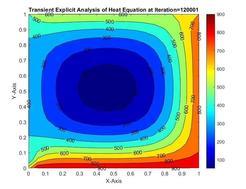
OUTPUT FOR EXPLICIT SOLUTION:

TRANSIENT STATE IMPLICIT SOLUTION:

%2D Temperature Transient Implicit Heat Conduction Equation 
clear all,close all,clc
%Number of nodes in each axis
nx=20;
ny=nx;
%Grid spacing based on nx and ny
x=linspace(0,1,nx);
y=linspace(0,1,ny);
dx=x(2)-x(1);
dy=y(2)-y(1);
%Time step input
dt=0.01;
%Thermal diffusivity of air
alpha=1.9e-5;
%A mesh is created with the x and y coordinates-matrix
[xx,yy]=meshgrid(x,y);
%Boundary Conditions
T=298.*ones(nx,ny);
T(1,:)=900;
T(end,:)=600;
T(:,1)=400;
T(:,end)=800;

%Rounding off corners for smooth simulation
T(1,1)=(400+900)/2;
T(1,ny)=(900+800)/2;
T(nx,1)=(400+600)/2;
T(nx,ny)=(600+800)/2;
%Input initial data as the 1st time step data
Told=T;
Tprev=T;
%Tolerance error and initial error is input
error_tol=1e-4;
initial_error=9e9;
%Constants based on the scheme are computed
k1=(alpha*dt)/(dx^2);
k2=(alpha*dt)/(dy^2);
K=1+(2*k1)+(2*k2);
%Omega for SOR computation is input
omega=1.2;
iterative_solver=3;
%Conditional statements for each method of implicit solution is input
if iterative_solver==1
    Tjacobi=jacobi_transient_implicit(initial_error,error_tol,T,Told,Tprev,xx,yy,nx,ny,k1,k2,K);
else if iterative_solver==2
    Tgauss=gauss_transient_implicit(initial_error,error_tol,T,Told,Tprev,xx,yy,nx,ny,k1,k2,K);
else if iterative_solver==3
    Tsor=sor_transient_implicit(initial_error,error_tol,T,Told,Tprev,xx,yy,nx,ny,k1,k2,K,omega);
end    
    end
end

FUNCTION FOR JACOBI METHOD:

%Function to solve 2D heat conduction equation implicitly using Jacobi method 
function T=jacobi_transient_implicit(initial_error,error_tol,T,Told,Tprev,xx,yy,nx,ny,k1,k2,K)
   %Iteration number is set to 1
   jacobi_iter=1;
   %A time loop is run for each time step for a computation after 20mins.
   for t=1:120000
      %After every time step computation error is set to initial error for
      %next computation
      initial_error=9e9;
      %A while loop is run for the convergence of solution based on error
      while(initial_error>error_tol)
          %Space loops in x and y are run for the computation of solution
          for i=2:nx-1
             for j=2:ny-1
                term1=1/K;
                term2=k1*term1; 
                term3=k2*term1;
                H=Told(i-1,j)+Told(i+1,j);
                V=Told(i,j-1)+Told(i,j+1);
                T(i,j)=(term1*Tprev(i,j))+term2*H+term3*V;
             end    
          end 
         %Error is calculated, and when it is higher than tolerance error, 
         %the loop repeats    
         initial_error=max(max(abs(Told-T)));
         %Told refers to the previous itration values and are updated after
         %each loop
         Told=T;
         jacobi_iter=jacobi_iter+1;
      end    
      %Tprev refers to temperature values at each time step, which are
      %updated after each time cycle
      Tprev=T;
   end
   %Plotting of 2D output
   figure(1)
   [a,b]=contourf(xx,yy,T);
   colormap(jet)
   colorbar
   title(sprintf('2D Transient Implicit Analysis of Heat Equation at Jacobi iteration=%d',jacobi_iter))
   xlabel('X-Axis')
   ylabel('Y-Axis')
   clabel(a,b)
end

OUTPUT FOR JACOBI METHOD:

FUNCTION FOR GAUSS SEIDEL METHOD:

%Function to solve 2D heat conduction equation implicitly using GS method 
function T=gauss_transient_implicit(initial_error,error_tol,T,Told,Tprev,xx,yy,nx,ny,k1,k2,K)
   %Iteration number is set to 1   
   gauss_iter=1;
   %A time loop is run for each time step for a computation after 20mins.
   for t=1:120000
      %After every time step computation error is set to initial error for
      %next computation
      initial_error=9e9;
      %A while loop is run for the convergence of solution based on error
      while(initial_error>error_tol)
          %Space loops in x and y are run for the computation of solution
          for i=2:nx-1
             for j=2:ny-1
                term1=1/K;
                term2=k1*term1; 
                term3=k2*term1;
                H=T(i-1,j)+Told(i+1,j);
                V=T(i,j-1)+Told(i,j+1);
                T(i,j)=(term1*Tprev(i,j))+term2*H+term3*V;
             end    
          end 
          %Error is calculated, and when it is higher than tolerance error, 
          %the loop repeats 
          initial_error=max(max(abs(Told-T)));
          %Told refers to the previous itration values and are updated after
          %each loop
          Told=T;
          gauss_iter=gauss_iter+1;
      end    
      %Tprev refers to temperature values at each time step, which are
      %updated after each time cycle
      Tprev=T;
   end
   %Plotting of 2D output
   figure(1)
   [a,b]=contourf(xx,yy,T);
   colormap(jet)
   colorbar
   title(sprintf('2D Transient Implicit Analysis of Heat Equation at GS iteration=%d',gauss_iter))
   xlabel('X-Axis')
   ylabel('Y-Axis')
   clabel(a,b)
end

OUTPUT FOR GAUSS SEIDEL METHOD:

FUNCTION FOR SOR METHOD:

%Function to solve 2D Heat conduction equation implicitly using SOR on the
%GS method
function T=sor_transient_implicit(initial_error,error_tol,T,Told,Tprev,xx,yy,nx,ny,k1,k2,K,omega)
   %Iteration number is set to 1  
   sor_iter=1;
   %A time loop is run for each time step for a computation after 20mins.
   for t=1:120000
      %After every time step computation error is set to initial error for
      %next computation 
      initial_error=9e9;
      %A while loop is run for the convergence of solution based on error
      while(initial_error>error_tol)
          %Space loops in x and y are run for the computation of solution
          for i=2:nx-1
             for j=2:ny-1
                term1=1/K;
                term2=k1*term1; 
                term3=k2*term1;
                H=T(i-1,j)+Told(i+1,j);
                V=T(i,j-1)+Told(i,j+1);
                Tsor=(term1*Tprev(i,j))+term2*H+term3*V;
                T(i,j)=(1-omega)*Tprev(i,j)+omega*Tsor;
             end    
          end 
          %Error is calculated, and when it is higher than tolerance error, 
          %the loop repeats
          initial_error=max(max(abs(Told-T)));
          %Told refers to the previous itration values and are updated after
          %each loop
          Told=T;
          sor_iter=sor_iter+1;
      end    
      %Tprev refers to temperature values at each time step, which are
      %updated after each time cycle
      Tprev=T;
   end
   %Plotting of 2D output
   figure(1)
   [a,b]=contourf(xx,yy,T);
   colormap(jet)
   colorbar
   title(sprintf('2D Transient Implicit Analysis of Heat Equation at SOR iteration=%d',sor_iter))
   xlabel('X-Axis')
   ylabel('Y-Axis')
   clabel(a,b)
end

OUTPUT FOR SOR METHOD:

CONCLUSION:

• In the steady state solution for solving 2D heat conduction equation, it is observed that the number of iterations follow the order `Jacobi>GS>SOR`. And similiarly, the time taken for the computation is proportional to the number of iterations. This can be explained because Jacobi method used the previous iteration values and converges to the solution. In the Gauss Seidel method, the solution converges faster because few data points are updated based on the current iteration, and in SOR method the convergence speed of the GS (used for this case) is increased by a factor `omega`. This applies to any case, the iteration number order stays the same, as in the next method, the data points chosen have a better solution than the previous iterations.
• In the transient state's explicit method, the number of iterations are less because the convergence step is skipped in each time loop. Based on the previous time step's data, the next time step data is calculated and the solution stops at the desired time.
• In the case of transient state implicit method, another while loop is input for the error calculation. This basically means that, the values for initial time step is guessed. And using the respective method, the while loop is executed, till an acceptable solution is reached. Once the acceptable solution is reached, the next time loop runs with these computed termperature values as the previous iteration's final solution.
• For each case, an arbitrary `omega=1.2` is used, But literature suggests based on the computation, there exists an ideal ωω value, which can be input to observe better solution, and faster convergence.
• The transient state solution as observed in the output has not converged yet. It is one of the transition states wherein the heat is still being discharged. Therefore, increase the number of time step iterations in the transient codes will lead to a converged steady solution.