Week 2 Air standard Cycle

Aim:

Solve otto cycle problem with python programing.

Objective:

1. Your code should create a PV diagram

2. You should output the thermal efficiency of the engine.

Theory:

The Otto cycle is the ideal cycle for spark-ignition reciprocating engines. In most spark-ignition engines, the piston executes four complete strokes (two mechanical cycles) within the cylinder, and the crankshaft completes two revolutions for each thermodynamic cycle. These engines are called four-stroke internal combustion engines.

Initially, both the intake and the exhaust valves are closed, and the piston is at its lowest position (BDC). During the compression stroke, the piston moves upward, compressing the air-fuel mixture. Shortly before the piston reaches its highest position (TDC), the spark plug fires and the mixture ignites, increasing the pressure and temperature of the system. The highpressure gases force the piston down, which in turn forces the crankshaft to rotate, producing a useful work output during the expansion or power stroke. At the end of this stroke, the piston is at its lowest position (the completion of the first mechanical cycle), and the cylinder is filled with combustion products. Now the piston moves upward one more time, purging the exhaust gases through the exhaust valve (the exhaust stroke), and down a second time, drawing in fresh air-fuel mixture through the intake valve (the intake stroke). Notice that the pressure in the cylinder is slightly above the atmospheric value during the exhaust stroke and slightly below during the intake stroke.

Equation Used:Various equations of Otto cycle are involved in this project. These are :

• Compression ratio (rc) , rc=(V1/V2)= 1+Vs/Vc
• Swept volume (Vs) = π/4⋅d^2⋅l, where d is bore diameter and l is stroke length,
• V/Vc = 1 + 1/2(rc−1)[R+1−cosθ−(R^2−sinθ^2)^1/2]

where R = length of connecting rod/crank radius ,

• Ideal Gas equation = p⋅v=m⋅R⋅T
• Thermal efficiency of Otto cycle(η)= 1−1/(r^γ−1)

Explanation:

• Since the otto cycle is an air standard cycle we will take the gamma value as 1.4.
• At the initial condition, we will consider the T1 and P1 values as 500K and 101.325KPa respectively.
• The geometrical parameters are stoke, diameter, connecting rod length, crank start and end angle are defined to the function in the program.
• From the above parameters, the v_c and v_s are calculated accordingly.
• The other states are calculated using adiabatic and ideal gas equations.
• Similarly, the thermal efficiency is calculated using the above formulas.
• For plotting p-v diagram plt.plot command is used from matplotlib.pyplot module.
• For the compression stage, the starting and ending crank angles are 180 and 0.
• For the expansion stage, the starting and ending crank angles are 0 and 180.
• Let us consider the value to be iterated is 50 accordingly v null set is created to store the value using append command.

Program:

import math
import matplotlib.pyplot as plt 
def engine_kinematics(bore,stroke,con_rod,cr,start_angle,end_angle):
	#engine parameters
	a = stroke/2
	R = con_rod/a
	v_s = (math.pi/4) * pow(bore,2) * stroke
	v_c = v_s/(cr -1)
	sc = math.radians(start_angle)
	ec = math.radians(end_angle)
	num_values = 50
	dtheta = (ec-sc)/(num_values - 1)
	v = []
	for i in range (0,num_values):
		theta = sc + i * dtheta
		term1 = 0.5*(cr-1)
		term2 = R+1-math.cos(theta)
		term3 = pow(R,2) - pow(math.sin(theta),2)
		term3 = pow(term3,0.5)
		v.append((1+term1*(term2-term3))*v_c)
	return v
#inputs 
p1 = 101325

t1 = 500

gamma = 1.4

t3 = 2300

#Geomentric parameter
bore = 0.1
stroke = 0.1
con_rod = 0.15
cr = 12

#volume computation
v_s = (math.pi/4) * pow(bore,2)*stroke
v_c = v_s/(cr-1)
v1 = v_s+v_c

#state point 2
v2 = v_c

#p2v2^gama = p1v1^gama
p2 = p1*pow(v1,gamma)/pow(v2,gamma)

#p2v2/t2 = p1v1/t1 | rhs = p1v1/t1 | p2v2/t2 = rhs
#t2 = p2v2/rhs
rhs = p1*v1/t1
t2 = p2*v2/rhs

v_compression  = engine_kinematics(bore,stroke,con_rod,cr,180,0)
constant = p1*pow(v1,gamma)
p_compression = []
for V in v_compression:
	p_compression.append(constant/pow(V,gamma))




#state point 3
v3 = v2

#p3v3/t3 = p2v2/t2 | rhs = p2v2/t2 | p3 = rhs *t3/v3
rhs = p2*v2/t2
p3 = rhs*t3/v3
v_expansion  = engine_kinematics(bore,stroke,con_rod,cr,0,180)
constant = p3*pow(v3,gamma)
p_expansion = []
for V in v_expansion:
	p_expansion.append(constant/pow(V,gamma))


# state point 4
v4 = v1

#p4v4^gama = p3v3^gamma
p4 = p3*pow(v3,gamma)/pow(v4,gamma)

#p4v4/t4 = rhs
t4 = p4*v4/rhs

plt.plot([v2,v3],[p2,p3])


plt.plot(v_compression,p_compression)

plt.plot(v_expansion,p_expansion)


plt.plot([v4,v1],[p4,p1])
plt.xlabel('volume')
plt.ylabel('pressure')
plt.title('pressure vs volume')


plt.show()

#thermal efficiency
thermal_efficiency = 1-(1/(pow(cr,(gamma-1))))
print ('Thermal efficiency is : ',thermal_efficiency)

Results:

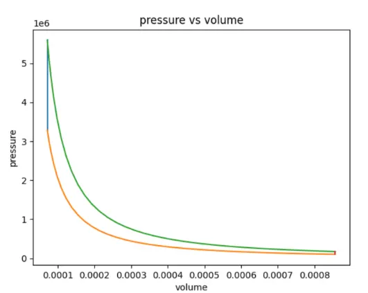
The cycle efficiency is around 63%