Week 3 - Solving second order ODEs

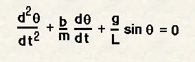
Aim : Write a program which can solve ordinary differential equation shown

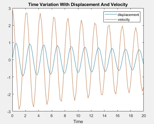
• Figure 1 : Plot a graph between displacement and velocity with respect to time.
• Figure 2 : Make a video to see motion of simple pendulum.

Variables : Here is the list of complete variable that is to be used further in this program.

• Length : This showes the length of the string used in simple pendulum. It has a unit of meter(m)and is specified as 'l' in this program.
• Mass : This is the total mass of the boob used in simple pendulum. It is specified in 'Kg' and is represented as 'm' in this program.
• Damping coefficient : Damping is an influence within or upon an oscillatory system that has the effect of reducing or preventing its oscillation. It is specified as 'b' in this program and this quantity is unitless.
• Gravity : Gravity is a natural phenomenon by which all things with mass or energy including planets, stars, galaxies, and even light are attracted to one another. The standard value of this gravity that we use is 9.81 m/s^2 and is specified as 'g'.

Program : Here there are two program first is the function program and the next one is main program.

Function Program : Save this in the same directory as that of the main program with the name 'ode.m'.

%Here we have made a function which will solve the given ode and give its result in [dtheta_dt]

function dtheta_dt = ode(t,theta,l,m,b,g)

% Variable are defined here
theta1=theta(1);
theta2=theta(2);

%The given ODE is broken into two first order differential equation to solve further
dtheta1_dt = theta2;
dtheta2_dt = -(b/m)*theta2-(g/l)*sin(theta1);

%The result of the two first order ODE will be saved now
[dtheta_dt] = [dtheta1_dt;dtheta2_dt];
end

Main Program : This is the main program and here we will call the function program with name 'ode' so it need to be saved with the same name.

clear all
close all
clc

%Input

t_span = linspace(0,20,100);
initials = [0 3];
l = 1;
m = 1;
b = 0.05;
g = 9.81;
ct=1;

%we have set our origin
x0=0;
y0=0;

%Here we have started for loop to take picture of all time for animation purpose

for i=1:length(t_span)
[t,result] = ode45(@(t,theta) ode(t,theta,l,m,b,g),t_span,initials);
theta = result(i,2);
x1=-l*sind(theta);
y1=-l*cosd(theta);
figure(1)
plot(x1,y1,'Marker','o','markersize',20,'markerfacecolor','r')
line([x0 x1],[y0 y1],'linewidth',4)

title('Simple Pendulum')
i = i+1;
axis([-1 1 -1.5 0])
M(ct)=getframe(gcf);
ct=ct+1;
pause(0.02)

end

%figure 2 will show the variation of dispacement and velocity w.r.t time.

figure(2)
plot(t,result(:,1))
hold on
plot(t,result(:,2))
legend('displacement','velocity')

title('Time Variation With Displacement And Velocity')

xlabel('Time')

%From here we have started making animation

video = VideoWriter('simple_pendulam _one.avi','uncompressed AVI');
open(video)
writeVideo(video,M);
close(video)

Result : Here is the variation graph of time w.r.t displacement and velocity.

Here is the link to access the animation : https://youtu.be/w_cCrbRZUto