Problem Set-1 c Week 11Challenge : Transient Handling
Problem:
The following table contains information about two vehicles
1. Calculate the following parameters for both using formulas
1. Undamped natural frequency (Hz)
2. Damping ratio
3. Damped frequency (Hz)
4. Rise time
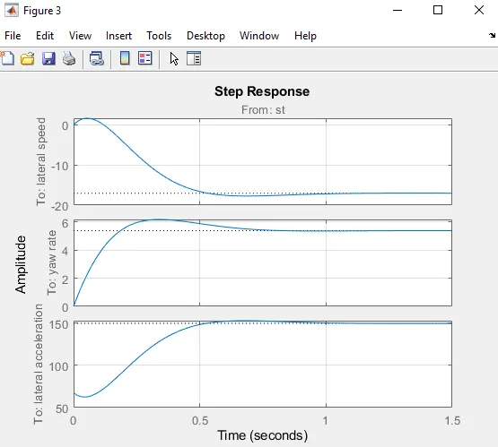
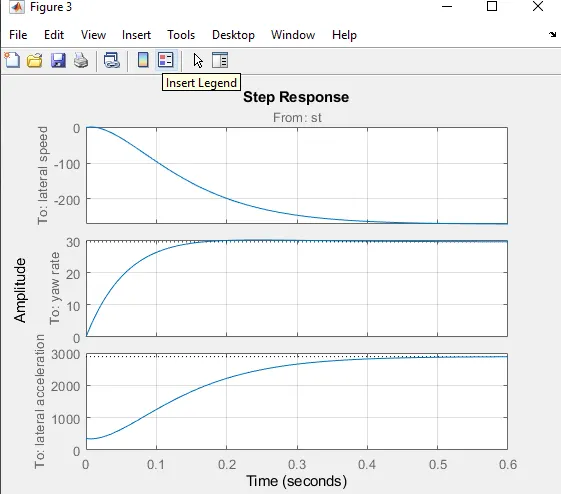
2. Plot the unit step response of the system for lateral speed, lateral acceleration and yaw rate
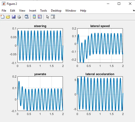
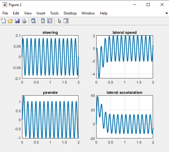
3. Plot the sine response of for lateral speed, lateral acceleration and yaw rate (5 deg, 7hz sine input)
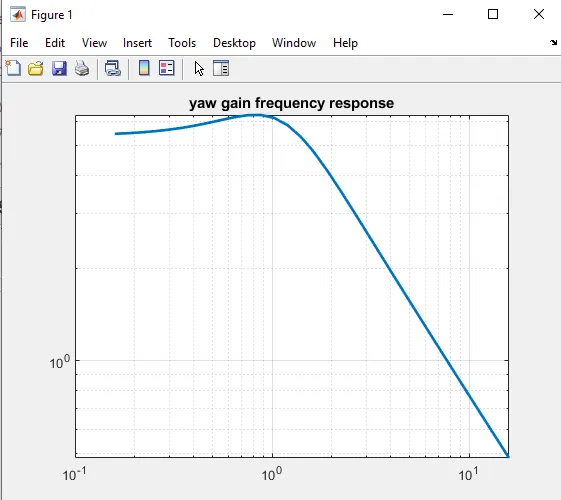
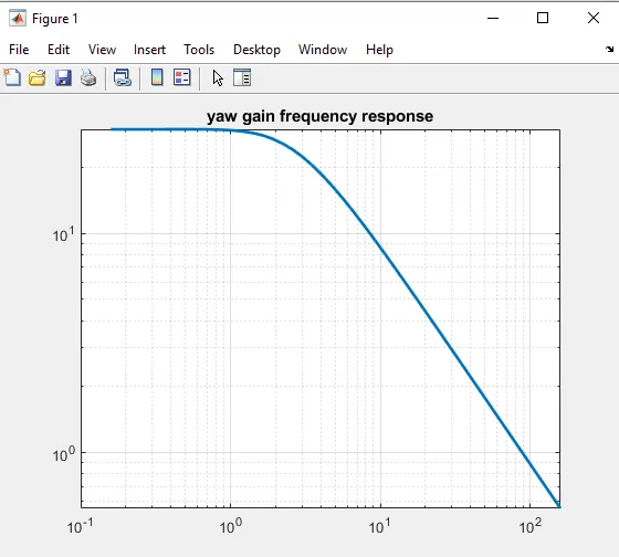
4. Plot the yaw gain (yaw/steering input) in the frequency domain
5. Show correlation for the following (in other words, you should get the same answer between two different methods of calculation)
1. Steady state yaw gain - between the sine response and the frequency response plot
2. Yaw gain at 7hz - between the sine reponse and the frequency response plot
3. Response time - between the step response plot and your analytical calculations
Answer:
Matlab Script: FWD Cars
clear all
close all
clc
% Wheelbase (m)
l = 2.538984 ;
% cg to front axle (m)
a = 0.890016;
% cg to rear axle (m)
b = l-a;
% Mass (kg)
m = 907.18474;
% moment of inertia (kg-m^2)
jz = 1128 ;
% front cornering stiffness (N/rad)
cf = 61171.9437;
% rear cornering stiffness (N/rad)
cr = 50976.6191;
% Speed m/s
u = 100/3.6;
A=[-(cf+cr)/(m*u),(((b*cr)-(a*cf))/(m*u))-u;((b*cr)-(a*cf))/(jz*u),-((((a^2)*cf)+((b^2)*cr))/(jz*u))];
B=[cf/m;(a*cf)/jz];
% Lateral Speed
c1=[1,0];
d1=0;
%Yaw rate
c2=[0,1];
d2=0;
%lateral acceleration
c3=A(1,:)+u*[0,1];
d3=B(1);
t=[0:0.01:2];
st=(pi/180)*5*sin(2*pi*7*t);
C=[c1;c2;c3];
D=[d1;d2;d3];
sys=ss(A,B,C,D);
Y=lsim(sys,st,t);
sys.Inputname={'st'};
sys.Outputname={'lateral speed','yaw rate','lateral acceleration'};
[mag1,phase1,omega1] = bode(sys({'yaw rate'},{'st'}));
for i=1:length(mag1);
magnitude1(i)=mag1(1,1,i);
i=i+1;
end
figure(1)
loglog(omega1/(2*pi),magnitude1,'linewidth',2)
title('yaw gain frequency response')
grid on
figure(2)
subplot(2,2,1)
plot(t,st,'linewidth',2)
title('steering')
grid on
subplot(2,2,2)
plot(t,Y(:,1),'linewidth',2)
title('lateral speed')
grid on
subplot(2,2,3)
plot(t,Y(:,2),'linewidth',2)
title('yawrate')
grid on
subplot(2,2,4)
plot(t,Y(:,3),'linewidth',2)
title('lateral accelaration')
grid on
figure(3)
step(sys)
grid on
S=stepinfo(sys);
[wn theta]=damp(sys);
% front cornering stiffness (N/rad)
Cf = -61171.9437;
Cr = -50976.6191
YB=Cf+Cr;
YR=(a*Cf-b*Cr)/u;
YS=-Cf;
NB=a*Cf-b*Cr;
NR=(((a^2)*Cf)+((b^2)*Cr))/u;
NS=-a*Cf;
%UnDamped Natural Frequency
Wn=sqrt(((YB*NR)+(NB*m*u)-(YR*NB))/(m*u*jz))
%Damping Ratio
Theta=abs(-((NR/jz)+(YB/(m*u)))*(1/(2*Wn)))
%Damped Frequency
Wd=Wn*sqrt(1-(Theta)^2)
%Rise Time
tr=((m*u*NS)/((YS*NB)-(YB*NS)))
Result:
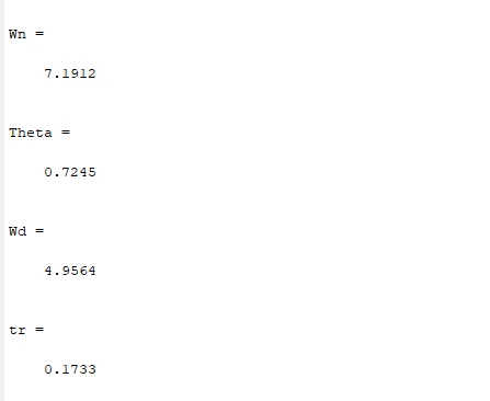
1.Undamped natural frequency = 7.2 rad/sec
2. Damping ratio = 0.72
3. Damped frequency = 4.95 rad/sec
4. Rise time = 0.173 sec
Matlab Script: F1 Racer
clear all
close all
clc
%Inputs
% Wheelbase (m)
l = 2.901696 ;
% cg to front axle (m)
a = 1.740408;
% cg to rear axle (m)
b = l-a;
% Mass (kg)
m = 779.725284;
% moment of inertia (kg-m^2)
jz = 865 ;
% front cornering stiffness (N/rad)
cf = 276803.935;
% rear cornering stiffness (N/rad)
cr = 429733.794;
% Speed m/s
u = 350/3.6;
A=[-(cf+cr)/(m*u),(((b*cr)-(a*cf))/(m*u))-u;((b*cr)-(a*cf))/(jz*u),-((((a^2)*cf)+((b^2)*cr))/(jz*u))];
B=[cf/m;(a*cf)/jz];
%lateral speed
c1=[1,0];
d1=0;
% yaw rate
c2=[0,1];
d2=0;
%lateral acceleration
c3=A(1,:)+u*[0,1];
d3=B(1);
t=[0:0.01:2];
st=(pi/180)*5*sin(2*pi*7*t);
C=[c1;c2;c3];
D=[d1;d2;d3];
sys=ss(A,B,C,D);
Y=lsim(sys,st,t);
sys.Inputname={'st'};
sys.Outputname={'lateral speed','yaw rate','lateral acceleration'};
[mag1,phase1,omega1] = bode(sys({'yaw rate'},{'st'}));
for i=1:length(mag1);
magnitude1(i)=mag1(1,1,i);
i=i+1;
end
figure(1)
loglog(omega1/(2*pi),magnitude1,'linewidth',2)
title('yaw gain frequency response')
grid on
figure(2)
subplot(2,2,1)
plot(t,st,'linewidth',2)
title('steering')
grid on
subplot(2,2,2)
plot(t,Y(:,1),'linewidth',2)
title('lateral speed')
grid on
subplot(2,2,3)
plot(t,Y(:,2),'linewidth',2)
title('yawrate')
grid on
subplot(2,2,4)
plot(t,Y(:,3),'linewidth',2)
title('lateral accelaration')
grid on
figure(3)
step(sys)
grid on
S=stepinfo(sys)
[wn theta]=damp(sys)
% front cornering stiffness (N/rad)
Cf = -276803.935;
Cr = -429733.794;
YB=Cf+Cr;
YR=(a*Cf-b*Cr)/u;
YS=-Cf;
NB=a*Cf-b*Cr;
NR=(((a^2)*Cf)+((b^2)*Cr))/u;
NS=-a*Cf;
%UnDamped Natural Frequency
Wn=sqrt(abs(((YB*NR)+(NB*m*u)-(YR*NB))/(m*u*jz)))
%Damping Ratio
Theta=abs(-((NR/jz)+(YB/(m*u)))*(1/(2*Wn)))
%Damped Frequency
Wd=Wn*sqrt(1-(Theta)^2)
%Rise Time
tr=abs((m*u*NS)/((YS*NB)-(YB*NS)))
Results:
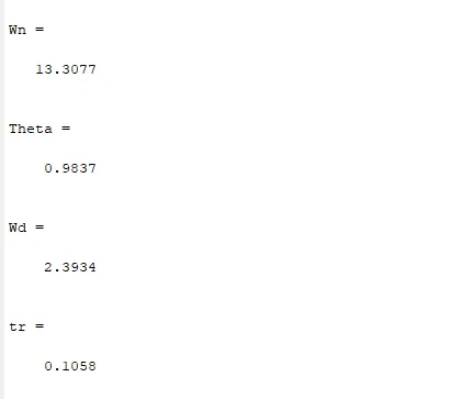
1.Undamped natural frequency = 13.30 rad/sec
2. Damping ratio = 0.98
3. Damped frequency = 2.39 rad/sec
4. Rise time = 0.10 sec