Week 4.1 - Genetic Algorithm
Aim:
- Write a code in MATLAB to optimise the stalagmite function and find the global maxima of the function.
- Clearly expalin the concept of genetic algorithm in your own words and also explain the syntax for ga in MATLAB in your report.
- Make sure that your code gives the same output, even if it is made to run several times.
- Plot graphs for all 3 studies and for F maximum vs no. of iterations. Title and axes labels are a must, legends could be shown if necessary.
Program:
1. This is the first section in which we will find the maximun value of the given problem.
1.a. First we need to write the given problem in a function and we need to save it in the same directory were we will save our main program.
function f = stalegamite(a)
p = (sin(5.1*pi*a(1)+0.5)).^6;
q = (sin(5.1*pi*a(2)+0.5)).^6;
c = ((a(1)-0.0667).^2)./0.64;
d = ((a(2)-0.0667).^2)./0.64;
r = exp(-4.*log(2).*c);
s = exp(-4.*log(2).*d);
f =-(p.*q.*r.*s);
end
1.b. From here we start our main program to find maximum value of the given problem.
clear all
close all
clc
% This is an input array(1D)
x = linspace(0,0.6,150);
y = linspace(0,0.6,150);
%This is used to make 2D array
[xx yy] = meshgrid(x,y);
for i=1:length(xx)
for j=1:length(yy)
a(1)=xx(i,j);
a(2)=yy(i,j);
f(i,j)=stalegamite(a);
end
end
surf(xx,yy,f)
xlabel('x values')
ylabel('y values')
shading interp
options=optimoptions('ga');
options=optimoptions(options,'populationsize',100)
[inputs,fval]=ga(@stalegamite,2,[],[],[],[],[0;0],[0.6;0.6],[],[],options)
Output:
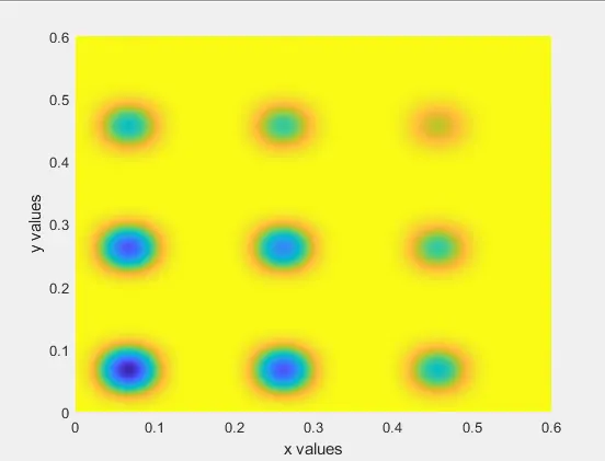
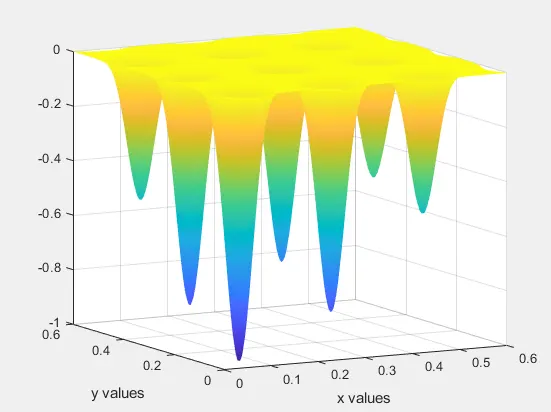
2.Concept of Genetic Algorithm: This is a tool that is used to optimize a given problem. Genetic algorithm is called as 'ga' in matlab. Genetic algorithm by default solves for minimum value of the given problem and to find maximum value we need to modify the function which contain the objective function. GA starts with random set values and and then moves toward the optimum value. This random set of values is called as population. Each individual of the population is called chromosome. In every iteration the value of chromosome changes and checked according to fitness function. To create next set of chromosome there are two ways to do that first is merging two chromosome using crossover operator and the second is modifing the chromosome using mutation operator. After several generation the chromosome converge to optimal solution.
3.Syntax of GA:
x=ga(fun,nvars) Here the function is 'fun' and 'nvars' is the number of variables in the function.
x=ga(fun,nvars,A,b,Aeq,beq) Here function is subjected to linear equalities.
x=ga(fun,nvars,A,b,Aeq,beq,lb,ub) Here the function is subjected to lower and upper bonds.
x=ga(fun,nvars,A,b,Aeq,beq,lb,ub,nonlcon,options)
4.Polt graph of all 3 studies.
4.A. Study 1 : Program
clear all
close all
clc
x=linspace(0,0.6,150);
y=linspace(0,0.6,150);
num_case=50;
[xx, yy]=meshgrid(x,y);
for i=1:length(xx)
for j=1:length(yy)
a(1)=xx(i,j);
a(2)=yy(i,j);
f(i,j)=stalegamite(a);
end
end
tic
for i=1:num_case
[inputs,fopt(i)]=ga(@stalegamite,2);
xopt(i)=inputs(1);
yopt(i)=inputs(2);
end
study1_time = toc
figure(1)
subplot(2,1,1)
surfc(x, y, f)
hold on
plot3(xopt,yopt,fopt)
xlabel('x values');
ylabel('y values');
zlabel('function values')
subplot(2,1,2)
plot(fopt)
xlabel('iteration');
ylabel('function values');
Outputs:
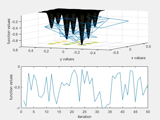

It took 4.9966 sec to run this program.Here the function values are between -1 and 0 and ga is changing function value in every run.
4.B. Study 2: Program.
clear all
close all
clc
x=linspace(0,0.6,150);
y=linspace(0,0.6,150);
num_case=50;
[xx, yy]=meshgrid(x,y);
for i=1:length(xx)
for j=1:length(yy)
a(1)=xx(i,j);
a(2)=yy(i,j);
f(i,j)=stalegamite(a);
end
end
tic
for i=1:num_case
[inputs,fopt(i)]=ga(@stalegamite,2,[],[],[],[],[0 0],[1 1]);
xopt(i)=inputs(1);
yopt(i)=inputs(2);
end
study2_time = toc
figure(1)
subplot(2,1,1)
surfc(x, y, f)
hold on
plot3(xopt,yopt,fopt)
xlabel('x values');
ylabel('y values');
zlabel('function values')
subplot(2,1,2)
plot(fopt)
xlabel('iteration');
ylabel('function values');
Output:
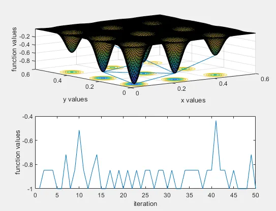

This took 7.7618 sec to run the program. Here we have reduced the range of function value and we are moving towards optimum solution.
4.C. Study 3: program
clear all
close all
clc
x=linspace(0,0.6,150);
y=linspace(0,0.6,150);
num_case=50;
[xx, yy]=meshgrid(x,y);
for i=1:length(xx)
for j=1:length(yy)
a(1)=xx(i,j);
a(2)=yy(i,j);
f(i,j)=stalegamite(a);
end
end
tic
options=optimoptions('ga');
options=optimoptions(options,'populationsize',200);
for i=1:num_case
[inputs,fopt(i)]=ga(@stalegamite,2,[],[],[],[],[0 0],[1 1],[],options)
xopt(i)=inputs(1);
yopt(i)=inputs(2);
end
study3_time = toc
figure(1)
subplot(2,1,1)
surfc(x, y, f)
hold on
plot3(xopt,yopt,fopt)
xlabel('x values');
ylabel('y values');
zlabel('function values')
subplot(2,1,2)
plot(fopt)
xlabel('iteration');
ylabel('function values');
Output:
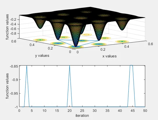

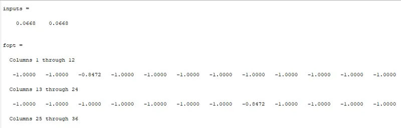 It took 18.4874 sec to run this program. here we added population size and we have managed our code to give global maximum value of function.